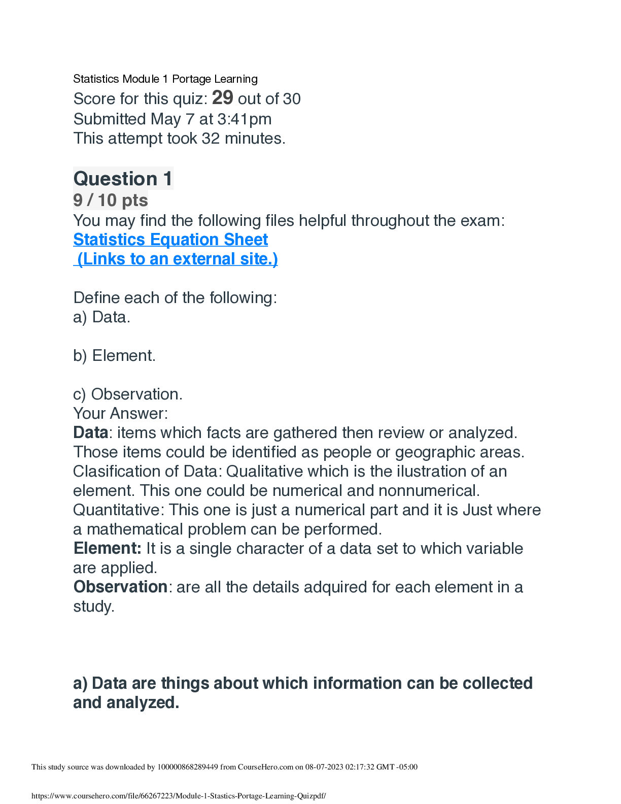
MATH 110 Module 1 Statistics Portage Learning Quiz (Latest Update) GRADED A
Statistics > STUDY GUIDE > New York UniversitySTAT-UB 0018Forecasting-HW-8. (All)
1) Time series plot of log(Rupee): 3.95 3.90 3.85 3.80 3.75 3.70 3.65 Date log(Rupee) TimeSeriesPlotof log(Rupee) ACF, PACF of the log series:1 10 20 30 40 50 60 70 80 90 1.0 0.8 0.6 0 ... .4 0.2 0.0 -0.2 -0.4 -0.6 -0.8 -1.0 Lag Autocorrelation AutocorrelationFunctionforlog(Rupee) (with5%significancelimitsfortheautocorrelations) 1 10 20 30 40 50 60 70 80 90 1.0 0.8 0.6 0.4 0.2 0.0 -0.2 -0.4 -0.6 -0.8 -1.0 Lag Partial Autocorrelation Partial AutocorrelationFunctionforlog(Rupee) (with5%significancelimitsforthepartial autocorrelations) Both plots indicate that the series needs to be differenced. ACF, PACF of the first-differenced log series:1 10 20 30 40 50 60 70 80 90 1.0 0.8 0.6 0.4 0.2 0.0 -0.2 -0.4 -0.6 -0.8 -1.0 Lag Autocorrelation AutocorrelationFunctionfor1dif(log(Rupee)) (with5%significancelimitsfortheautocorrelations) 1 10 20 30 40 50 60 70 80 90 1.0 0.8 0.6 0.4 0.2 0.0 -0.2 -0.4 -0.6 -0.8 -1.0 Lag Partial Autocorrelation Partial AutocorrelationFunctionfor1dif(log(Rupee)) (with5%significancelimitsforthepartial autocorrelations) The ACF and PACF of the first-differenced log series indicates that an ARIMA (0,1,0) model would be appropriate for the log series.2) In this case, ARIMA(2,1,2) with no constant is chosen because it has the lowest AICC value: ARIMA Models (no constant) p d q SS AICc 0 1 0 0.0460871 -24100.11301 1 1 0 0.0459824 -24103.19037 2 1 0 0.0459771 -24101.44249 0 1 1 0.0459849 -24103.06891 1 1 1 0.045979 -24101.49594 2 1 1 0.045971 -24099.73172 0 1 2 0.045976 -24101.49594 1 1 2 0.0459702 -24099.7706 2 1 2 0.04572 -24109.95372 Forecasts from period 2235 95% Limits Period Forecast Lower Upper Actual 2236 3.78650 3.77762 3.79538 3)-0.06 -0.04 -0.02 0.00 0.02 99.99 99 90 50 10 1 0.01 Residual Percent 3.7 3.8 3.9 4.0 0.02 0.00 -0.02 -0.04 -0.06 Fitted Value Residual -0.0625 -0.0500 -0.0375 -0.0250 -0.0125 0.0000 0.0125 0.0250 800 600 400 200 0 Residual Frequency 0.02 0.00 -0.02 -0.04 -0.06 ObservationOrder Residual Normal Probability Plot VersusFits Histogram VersusOrder Residual Plotsforlog(Rupee) 0.04 0.02 0.00 -0.02 -0.04 -0.06 Date RESI1 TimeSeriesPlotof RESI10.004 0.003 0.002 0.001 0.000 Date RESI1^2 TimeSeriesPlotof RESI1^2 [Show More]
Last updated: 3 years ago
Preview 1 out of 13 pages

Buy this document to get the full access instantly
Instant Download Access after purchase
Buy NowInstant download
We Accept:

Can't find what you want? Try our AI powered Search
Connected school, study & course
About the document
Uploaded On
Apr 27, 2021
Number of pages
13
Written in
All
This document has been written for:
Uploaded
Apr 27, 2021
Downloads
0
Views
49
Scholarfriends.com Online Platform by Browsegrades Inc. 651N South Broad St, Middletown DE. United States.
We're available through e-mail, Twitter, Facebook, and live chat.
FAQ
Questions? Leave a message!
Copyright © Scholarfriends · High quality services·