# Week 5 Notes Variable Selection, Georfia Tech, Graded A+

Document Content and Description Below

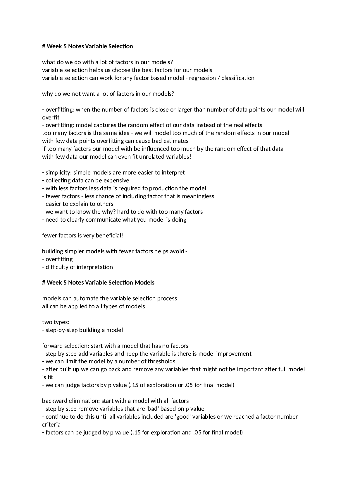
# Week 5 Notes Variable Selection what do we do with a lot of factors in our models? variable selection helps us choose the best factors for our models variable selection can work for any factor ba ... sed model - regression / classification why do we not want a lot of factors in our models? - overfitting: when the number of factors is close or larger than number of data points our model will overfit - overfitting: model captures the random effect of our data instead of the real effects too many factors is the same idea - we will model too much of the random effects in our model with few data points overfitting can cause bad estimates if too many factors our model with be influenced too much by the random effect of that data with few data our model can even fit unrelated variables! - simplicity: simple models are more easier to interpret - collecting data can be expensive - with less factors less data is required to production the model - fewer factors - less chance of including factor that is meaningless - easier to explain to others - we want to know the why? hard to do with too many factors - need to clearly communicate what you model is doing fewer factors is very beneficial! building simpler models with fewer factors helps avoid - - overfitting - difficulty of interpretation # Week 5 Notes Variable Selection Models models can automate the variable selection process all can be applied to all types of models two types: - step-by-step building a model forward selection: start with a model that has no factors - step by step add variables and keep the variable is there is model improvement - we can limit the model by a number of thresholds - after built up we can go back and remove any variables that might not be important after full model is fit - we can judge factors by p value (.15 of exploration or .05 for final model) backward elimination: start with a model with all factors - step by step remove variables that are 'bad' based on p value - continue to do this until all variables included are 'good' variables or we reached a factor number criteria - factors can be judged by p value (.15 for exploration and .05 for final model)stepwise regression: combination of forward selection and backward elimination - start with all or no variables - at each step add or remove a factor based on some pvalue criteria - model will adjust older factors based on what new values we add to the model - we can use other metrics AIC, BIC, R^2 to measure 'good' variables in any step by step method step-by-step = greedy algorithm, does the one step that is the best without taking future options into account - these are model 'classical' newer methods based on optimization models that look at all possible options at the same time - LASSO: add a constraint to the standard regression equation to bound coefficients from getting large - sum of the coefficients sumof(|ai|) <= t - regression has a budget t to use on coefficients - factors that are not important will be dragged down to 0 - constraining any variables means we need to scale the data beforehand! - how to be pick t? - number of variables and quality of model? - try LASSO with different values of t and choose the best performance - Elastic Net: combination of LASSO and RIDGE regression - constrain a combination of the absolute value of the sum of coefficients vs. the squared sum of coefficients - need to scale the data - sumof(ai^2) <= t - without the absolute term we have RIDGE regression - these are global approaches to variable selection what is the key difference between stepwise and LASSO regression? - lasso has a regularization term and requires the data to be scaled beforehand - in regression contexts LASSO needs to be scaled - size constraint will pick up the wrong values because magnitude of factors messes with the coefficient estimates! # Week 5 Notes variable selection - greedy variable selection - stepwise - global optimization - LASSO, ridge, Elastic net how do we choose between these methods? stepwise methods: good for exploration and quick analysis - stepwise is the most common - can give set of variables that fit to random effects - they might generalize as well to new data global optimization: slower but better for prediction - LASSO, Elastic NetRegularized Regression: LASSO: - minimize sumof((yi - (a0 _ a1x1 + a2x2 + ... + ajxji))^2) subject to sumof(|ai|) <= t - some coefficients forced to zero to simplify model - will take some variables to zero but they may not be the ones we want! - with correlated variables, LASSO will only keep one but it not be 'right' in terms of cost or interpretation RIDGE: - minimize sumof((yi - (a0 _ a1x1 + a2x2 + ... + ajxji))^2) subject to sumof(ai^2) <= t - coefficients shrink toward 0 to reduce variance in estimate (never get to 0) - important coefficients will be shrunk - this might give higher bias in hopes of better variance performance - really good predictors might be underestimated by this method Elastic Net: - minimize sumof((yi - (a0 _ a1x1 + a2x2 + ... + ajxji))^2) subject to lambda * sumof(|ai|) + (1- lambda)*sumof(ai^2) <= t - elastic net is LASSO regression plus RIDGE regression - quadratic term shrinks the coefficient values - regularized close to 0 - shrinking the coefficients give bias but reduces variance - trading off bias to variance can lead to model improvement - remember: performance is reducing bias and variance! - Elastic Net gets the selection benefits of LASSO with the predictive benefits of RIDGE! - Elastic Net also gets some of the drawbacks for both models as well - Elastic Net will arbitrarily rule out some correlated variables like LASSO - Elastic Net will underestimate coefficients of very predictive variables like RIDGE try many different versions and compare the results models provide insight and direction but need to decide on all inputs # Week 5 Notes Experiment Design introduction to design of experiments - we assumed we already have data - data can be easily collected - this is not the case... - getting the full set of data is impossible or will take too long - we need: DOE collect best subset quickly and efficiently - need to make sure the data we get will be sufficient to answer our questions - how to make our data representative of all our factors? Design of Experiments (DOE) - comparison and control: compare two things but need to control for other factors - need to match across comparisons across other factors than the study we are setting up - need to control for the effects of our other variables - data has the same mix - or breakdown the data into smaller sets to test all important factors- blocking: creating variation - type is a blocking factor that we can account for - we want to reduce the variability by eliminating variation on certain factors - sports cars more likely to be red - analyze red sports cars and red family cars in separate sets to reduce variance # Week 5 notes A / B Testing - use analytics to pick the best set of different alternatives - using design of experiments to A / B test - collect some data - randomly serve up ads and track how they are clicked - we will have binomial ads based on clicks for each banner add - we can use a basic hypothesis test to determine which add is better - can do hypothesis testing on the fly - this is A / B testing: choosing between two alternatives to do A / B testing we need to satisfy these three things: 1. collect data quickly (lots of data) 2. data must be representative of entire population 3. data must be small compared to the whole population (need a smaller slice of the total traffic) - common approach in marketing - what about several alternatives? - how do we figure out the best alternative? - we don't want to waste trials on bad alternatives - how do we manage this? - how to be test multiple factors accounting for our 'budget' of possible test cases? # Week 5 Notes Factorial Design A / B testing - compare between simple alternatives Factorial Design: what factors are import? - test effectiveness of every combination in our ads (full factorial design) - after testing them all - basic anova can tell which are important - testing combinations quickly scales outside the realm of possibility (fractional factorial design) - limit the tests to a subset of important subsets first then test to see most important factors design depends on data - fractional experiment design might be more feasible - we can cleverly design our choices to be 'representative' of all different options - i.e. test attributes across the minimum number of cases to get full representation of each choice - balanced design: - test each choice the same number of times - test each pair of choices the same number of times - good designs are essential to creating a representative test - independent factors: - test subset of combinations - use regression to estimate effects- regression can model the response as 'clicks' based on each of the factors included (if independent factors) Key Takeaway: - all of these DOE methods can be helpful when they are used for modeling or even before the data is collected! - factorial design can be a powerful tool to determine the best comparisons to make and explain the results of the final choices # Week 5 Notes Multi-Armed Bandit determine the better of two alternatives - AB testing - try it out an test which is better - hypothesis test - we can also test factors in factorial design exploration vs. exploitation - there is a cost for each test - we may be losing value - the number of tests can be wasted on tests - say we find after 1000 tests that option A was the best: all tests with option B would have been wasted - these wrong adds are lost value - trade off between being sure are losing value in testing - balance benefits from more information vs. getting more value - this is exploration vs. exploitation - exploration - certainty in knowing the correct answer - exploitation - maximizing immediate value - this is the multi-armed bandit problem - slot machine = one armed bandit (negative expected value) - several slot machines = different expected payout - only way to find out is to test them all - multi-armed bandit: - start with k alternatives: - start with no information - equal probability of selecting each alternative - run some tests and gather some information - update our probabilities based on our initial tests - then assign new tests skewed towards the new probabilities - we are testing multiple options so we are still exploring... - but we are skewing our tests to try and take advantage of exploitation - do this until answer is absolutely clear of the best case - it might take longer to get to the clear answer but we will have attempted to maximize value by shifting choice to the 'hot' choice in terms of success - MAB parameters - # of tests between recalculating probabilities - how to update our probabilities of success - change how we assign new tests no simple rule but works better than fixed large number of tests - worthwhile: learn faster on the fly and create more value# Week 5 Notes Probability Distributions probability distributions - sometimes simple approaches work better - can use simple probability distributions instead of modeling a bunch of factors - probability models can model certain problems that allow us to 'skip' factor based modeling - matching data to a probability distribution can give insight - important when we only have the response or hard to get new data focus on which distributions will be good for modeling: Bernoulli: more flexible coin flip p = 'heads' 1 - p = 'not heads' can model any event - very useful when we string the event probabilities together - Bernoulli trials - the probability p of our event stays the same from time period to time period - test: observe successes and use the distribution to see what the probability is to get that same number of successes - this is the binomial distribution: we can examine the probability mass function - probability of getting x successes out of n independent identically distributed Bernoulli trials - binomial distribution converges to normal distribution - P(X = x) = (n x) p^x(1 - p)^n-x - as n gets very large the binomial distribution converges to the normal distribution - normal distribution is useful for predicting errors Geometric Distribution: - PMF: P(X = x) = (1-p)^x * p - probability of having x bernoulli(p) failures until first success - or flipped, x bernoulli (1 - p) successes until first failure - we have to be careful of how we define p and 1-p in this distribution - we can compare data to geometric to test whether i.i.d is true - if something fits the geometric distribution then we can assumme i.i.d will hold - this is a way to check if an outcome is actually being treated as independent! Poisson Distribution: - fx(x) = lambda^x * e^-lambda / x! - good at modeling random arrivals - lambda is the average number of arrivals - probability x people arrive given lambda (average arrival rate) - this assumes that arrivals are independent and identically distributed (i.i.d) Exponential Distribution: - related to the poisson distribution - models the inter-arrival time - if arrivals are poisson with lambda arrival average time - the time between successive arrivals is an exponential distribution (lambda) - poisson arrivals = exponential inter-arrivals time and vice versa - PMF: fx(X) = lambda * e^-lambda*x - 1 / lambda is the average inter-arrival timeWeibull Distribution: - amount of time it takes for something to fail - similar to geometric exempt time passed instead of instances - PMF = fx(x) = k / lambda * (x / lambda)^k-1 * e^-(x/lambda)^k - lightbulb: how many flips before failure = geometric - lightbulb: how long to leave lightbulb on before failure = Weibull - additional parameter k - K < 1 = models when failure rate decreases with time 'worse things fail first' - K > 1 = models when failure rate increases with time 'things that wear out' - K = 1 = failure rate is constant with time - when k = 1 weibull reduces to exponential distribution how do we tell is our data fits one of these distributions? - fit to best distribution and give the best fit parameters for the fit = software - can also fit to many different models at once to figure out the best distribution - warning: only use software as guide - data may have random noise in it - think about what the output means before using it! # Week 5 Notes Q-Q Plots probability based models: -visualize whether two distributions are the same - see if data is similar to a distribution - visualization is important to see what the software is outputting Q-Q Plot: - idea of this plot is that whatever variations in the data - even if the number of data points in two sets is very different... - two similar distributions should have about the same value at each quantile - ex. in each of the two datasets the value that at the 10th percentile should be close to the same for each distribution - this should be true at any percentile if the distributions are similar - the q-q plot show this graphically - plot median vs. median for each distribution - do this for all percentiles - sample 1 vs. sample 2 - want a 45 degree line to say that the distributions match - this would be the same as a statistical test - but the plot let's us see why (where are the distributions different) - raw statistical test can be misleading (small tail differences) - we can compare two datasets or just one dataset to compare to a other distribution - compare the actuals to the 'perfect' simulated distribution to see if there is a good match # Week 6 Notes Queuing - using distributions to model queues Example: - autodialer automatically calls phone numbers - if the call is answered it is put into a queue - how many employees should we have? - based on how many people will answer the autodialer- based on duration of call once the employee is on the phone this can be analyzed based on a queuing system - calls are answered and added by a probability distribution - we have c number of employees - calls leave the system based on another probability distribution Example: - call start is Poisson (lambda) - 1 employee - call end is Exponential (u) time - we can calculate: - expected fraction of time employee is busy - expected waiting time before talking to employee - expected number of calls waiting in queue Transition Equations to Model the Process: - Arrival Rate (calls) = lambda - Service Rate (calls) = u > lambda - Transition Equations (>= 1 calls in queue) P(next event is an arrival) = lambda / (lambda + u) P(next event is a finished call) = u / (lambda + u) - Can calculate: Expected fraction of time employee is busy = lambda / u Expected waiting time before talking to employee = lambda / u(u - lambda) Expected number of calls waiting in queue = lambda^2 / (u(u - lambda)) [Show More]

Last updated: 3 years ago

Preview 1 out of 28 pages