
Rasmussen College NUR201 MDC4 Exam1 ONLY correct answers are provided.
$ 9
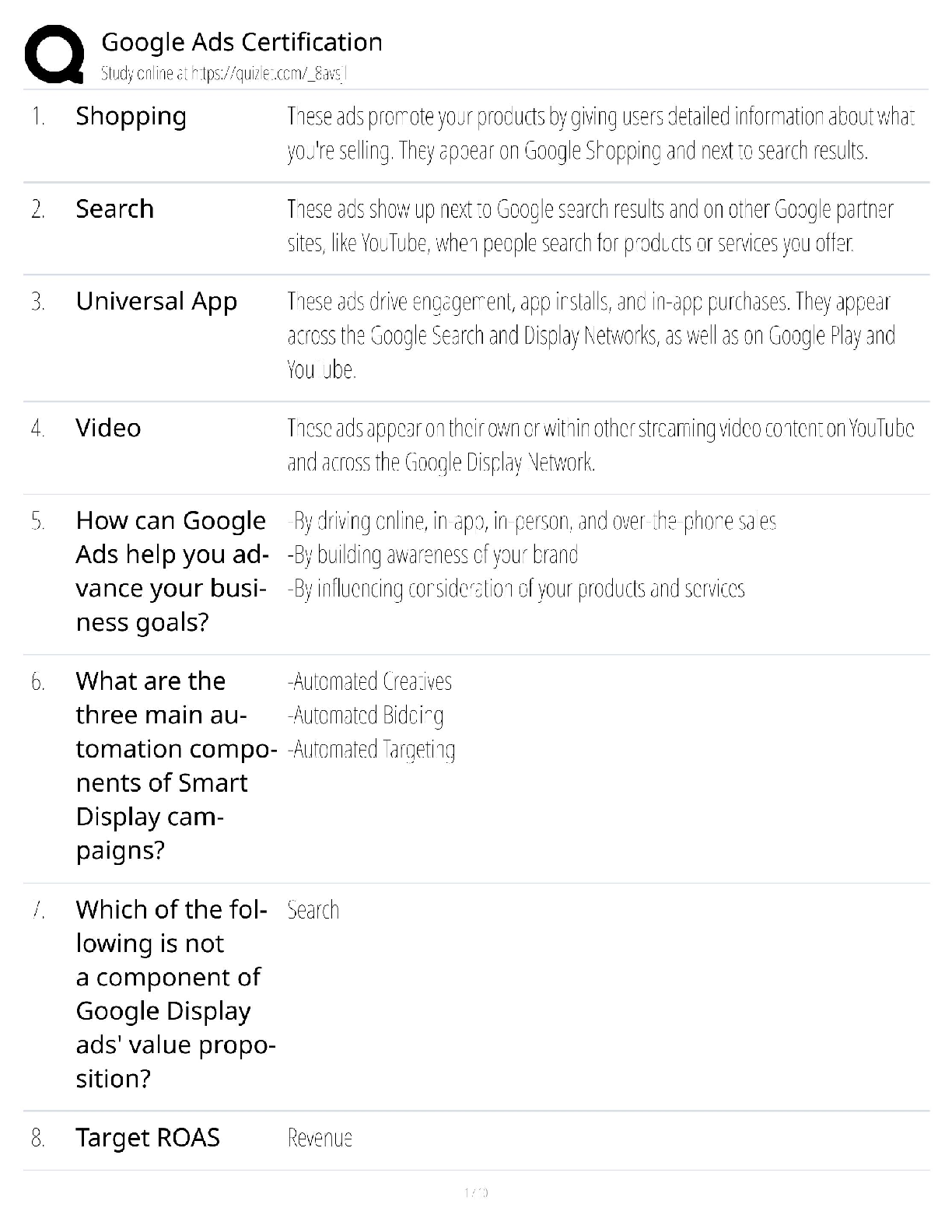
MKTG 455 Google Ads Certification Guide / Search, Display & Video Exams / 2025 Study Hub & Test Bank / Score 100%
$ 28.5
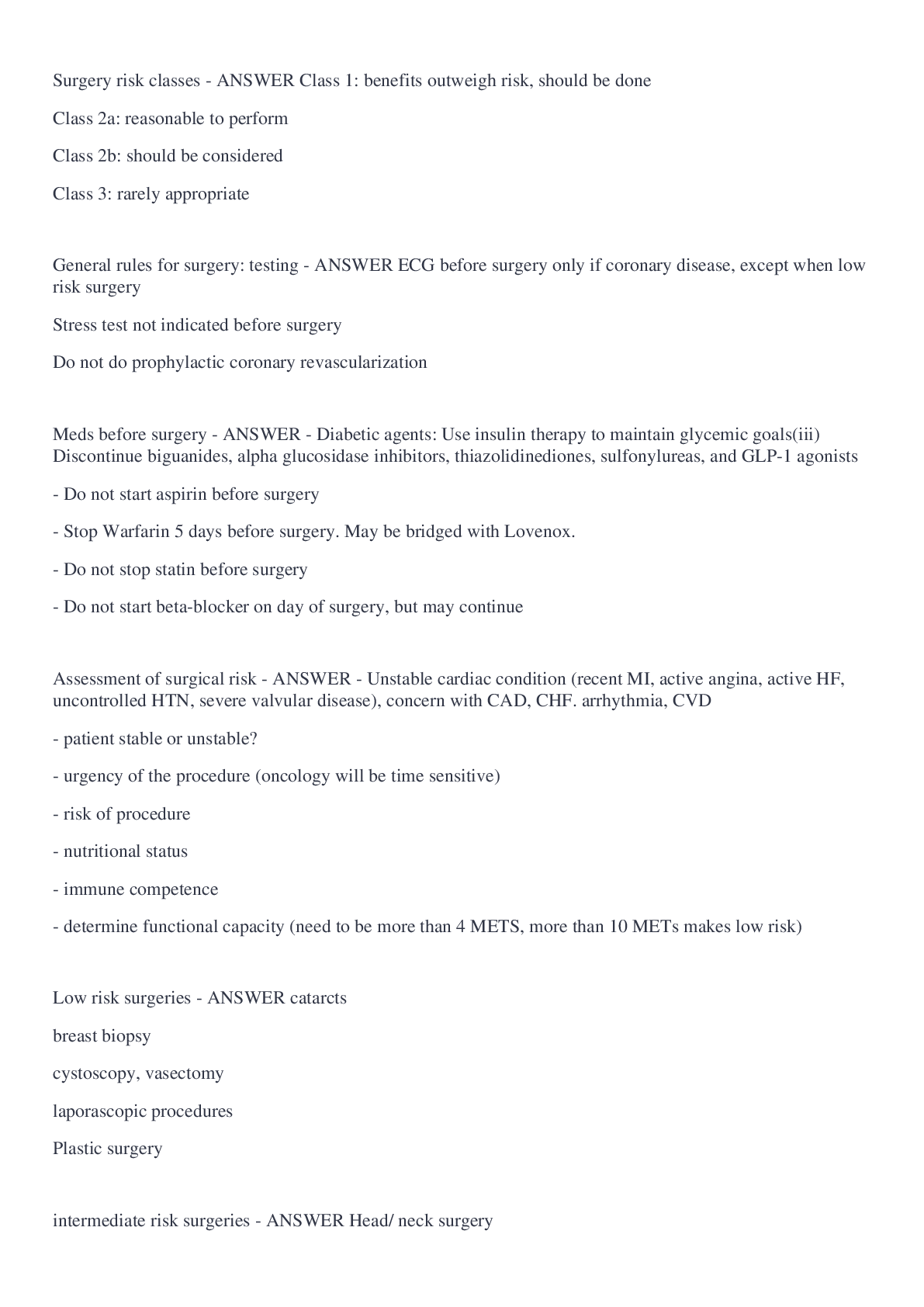
PRIMARY CARE TESTBANK THE ART AND SCIENCE OF ADVANCED PRACTICE NURSING - AN INTERPROFESSIONAL APPROACH 6TH EDITION
$ 24

Pearson Edexcel International GCSE (9–1) || Computer SciencePaper 2: Application of Computational Thinking || QUESTION PAPER 2019
$ 6
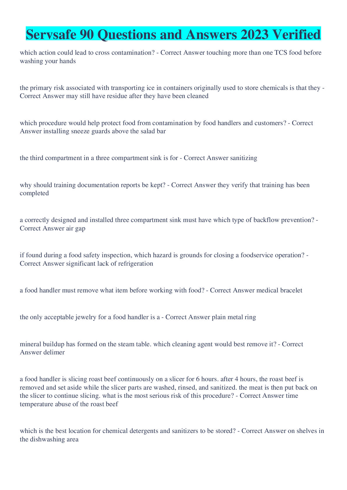
Servsafe 90 Questions and Answers 2023 Verified
$ 8
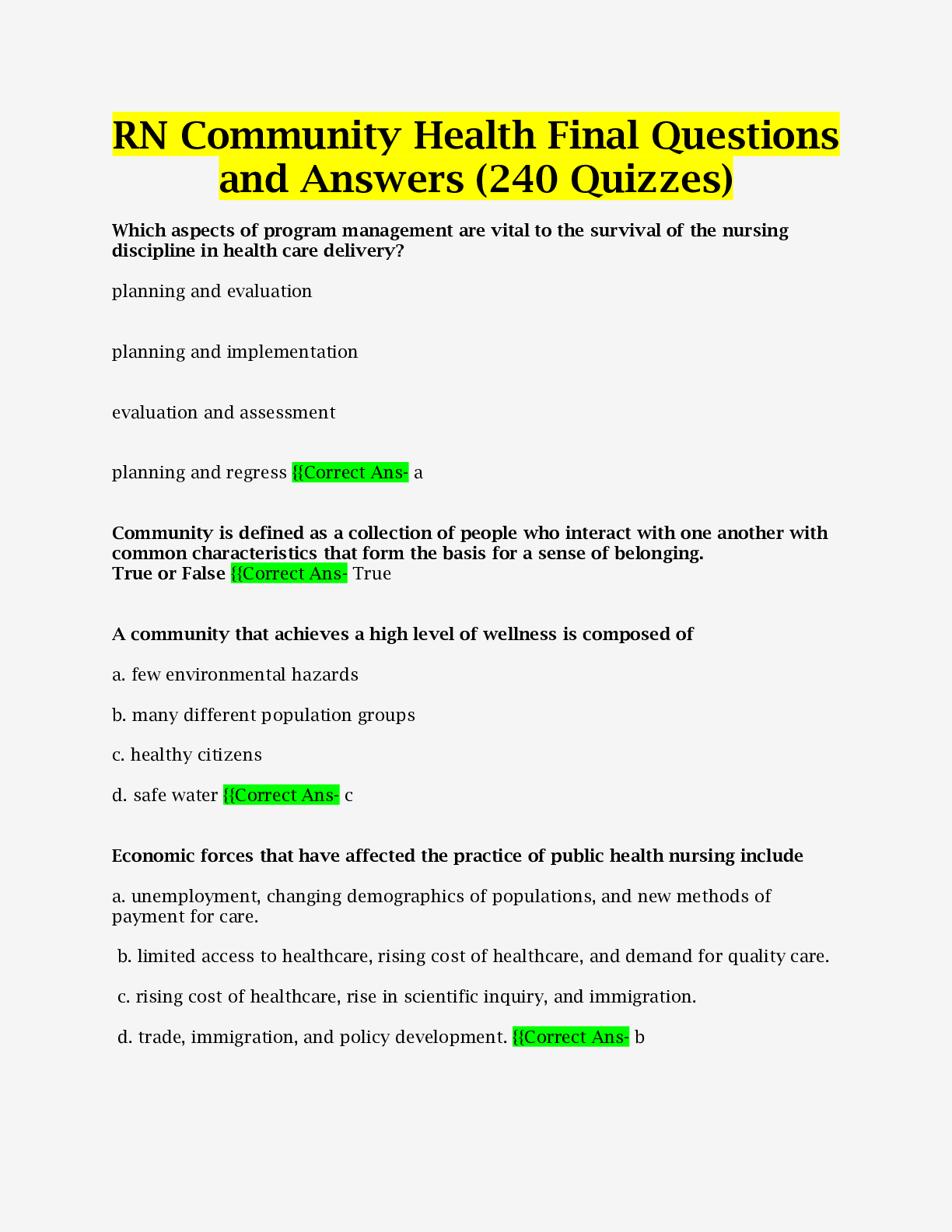
RN Community Health Final Questions and Answers (240 Quizzes) |Guarantee A+ Score
$ 10
NUR 304 Exam 1 Test Bank; Varcarolis’ Foundations of Psychiatric Mental Health Nursing. GRADED A, QUESTIONS WITH CORRECT ANSWERS
$ 25
eBook Data Smart Using Data Science to Transform Information into Insight 2nd Edition by Jordan Goldmeier
$ 29

LECTURE NOTES & SOLUTIONS for Data Mining and Machine Learning: Fundamental Concepts and Algorithms 2nd Edition by Mohammed J. Zaki, Wagner Meira Jr
$ 19

Elevator Mechanics Final Exam – 137 Questions And Answers
$ 15
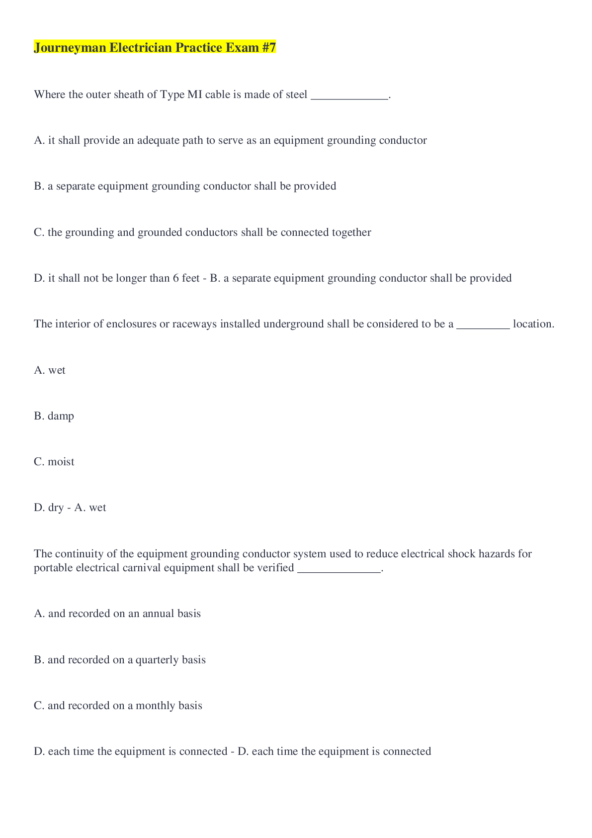
Journeyman Electrician Practice Exam #7 questions well verified
$ 13

Administrative Law- Bureaucracy in a Democracy 6th Edition Daniel E. Hall INSTRUCTORS SOLUTION MANUAL
$ 20.5
UNIV 104 Math Assessment Part 1 Part 2 Liberty University answers & Complete solutions
$ 13
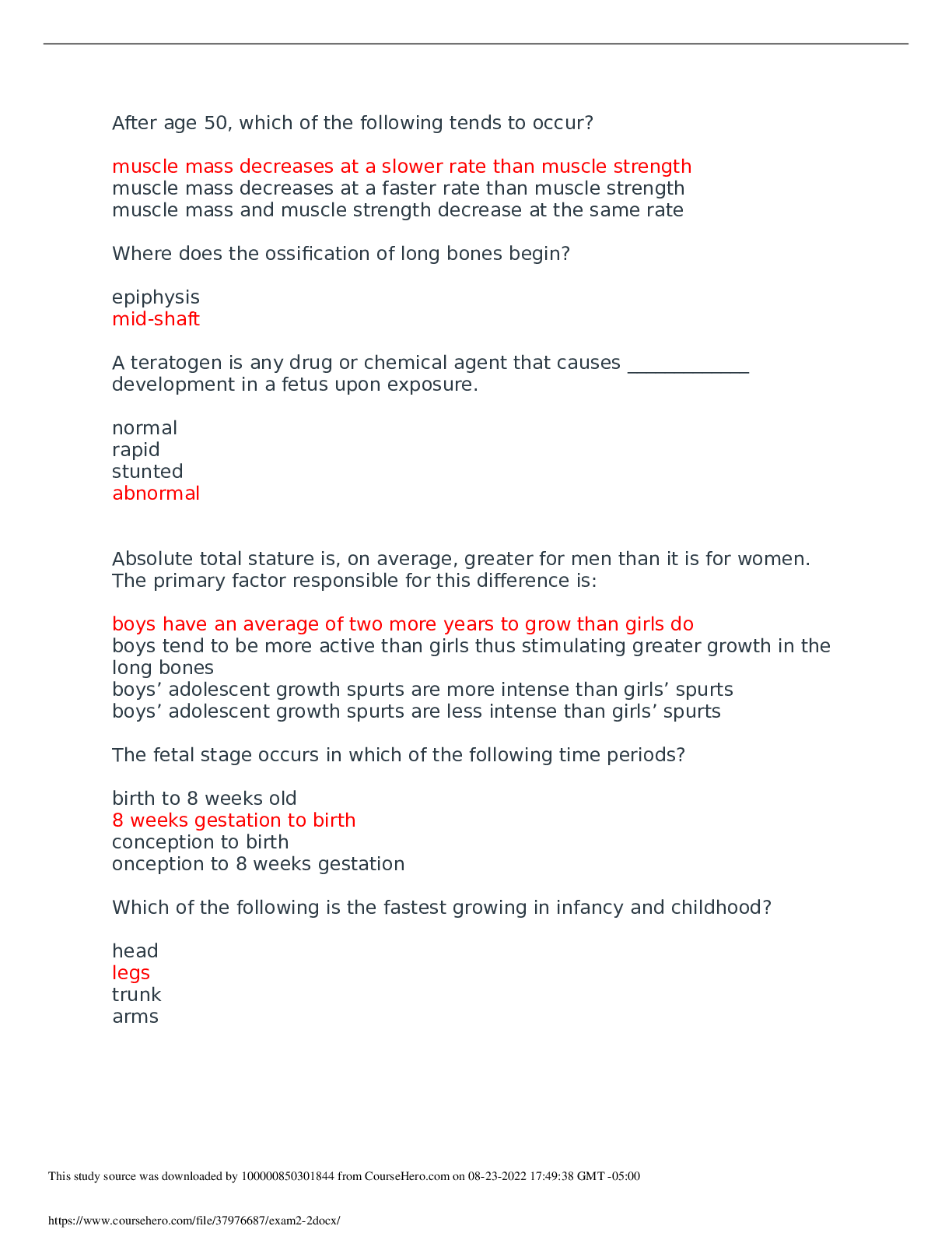
Questions and Answers > California State University, Northridge KIN 477 Developmental Exam 2-2
$ 8
ATI RN Comprehensive Predictor 2019 Form A
$ 6
Case Notes/Answers Deloitte Recommends Client Selection to Regency Bank, By Mehmet Begen, Stacey Yue
$ 45
NRNP 6560 Midterm exam with complete solutions
$ 10
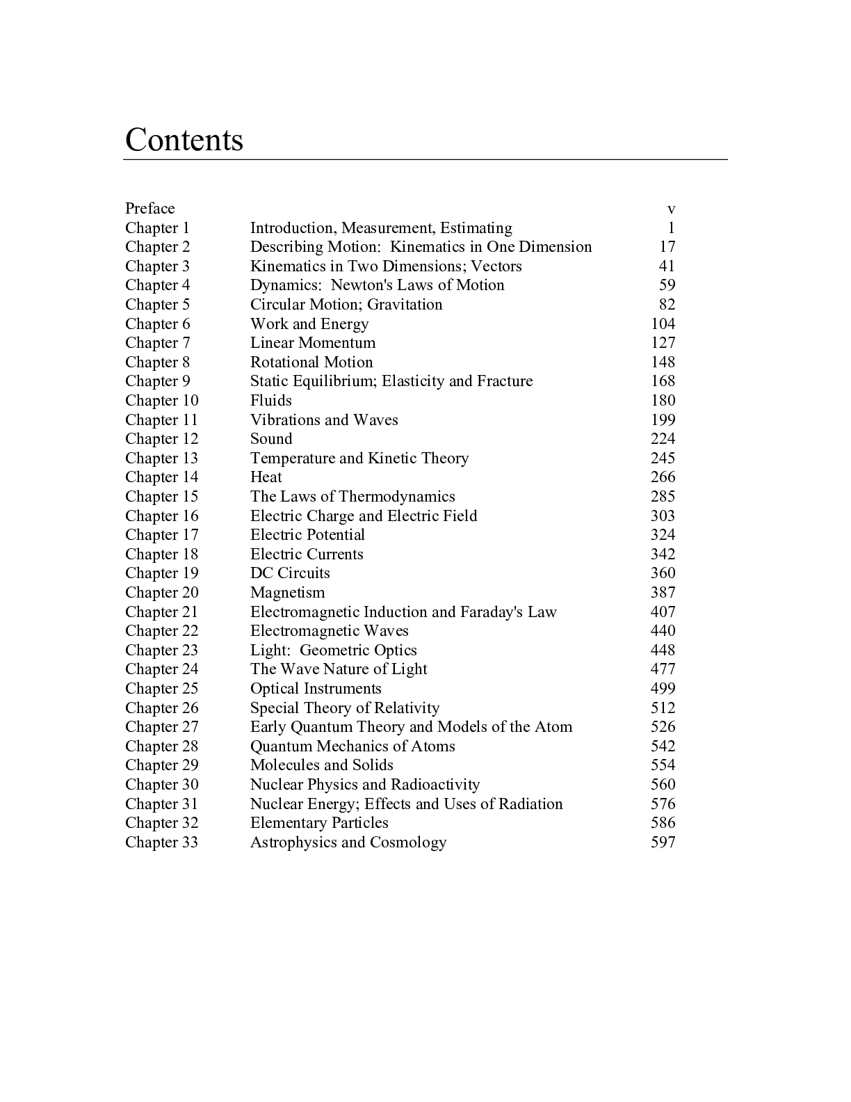
Test Bank for Physics Principles with Applications by Douglas C. Giancoli
$ 20
HESI PEDIATRICS PRACTICE EXAM/ Latest 2022/ Complete A+Guide


