14.1 Functions of Several Variables
1. (a) From Table 1, (−1540) = −27, which means that if the temperature is −15◦C and the wind speed is 40 kmh, then the
air would feel equivalent to approximately −27◦C without wi
...
14.1 Functions of Several Variables
1. (a) From Table 1, (−1540) = −27, which means that if the temperature is −15◦C and the wind speed is 40 kmh, then the
air would feel equivalent to approximately −27◦C without wind.
(b) The question is asking: when the temperature is −20◦C, what wind speed gives a wind-chill index of −30◦C? From
Table 1, the speed is 20 kmh.
(c) The question is asking: when the wind speed is 20 kmh, what temperature gives a wind-chill index of −49◦C? From
Table 1, the temperature is −35◦C.
(d) The function = (−5 ) means that we fix at −5 and allow to vary, resulting in a function of one variable. In
other words, the function gives wind-chill index values for different wind speeds when the temperature is −5◦C. From
Table 1 (look at the row corresponding to = −5), the function decreases and appears to approach a constant value as
increases.
(e) The function = ( 50) means that we fix at 50 and allow to vary, again giving a function of one variable. In
other words, the function gives wind-chill index values for different temperatures when the wind speed is 50 kmh . From
Table 1 (look at the column corresponding to = 50), the function increases almost linearly as increases.
2. (a) From Table 3, (9570) = 124, which means that when the actual temperature is 95◦F and the relative humidity is 70%,
the perceived air temperature is approximately 124◦F.
(b) Looking at the row corresponding to = 90, we see that (90 ) = 100 when = 60.
(c) Looking at the column corresponding to = 50, we see that (50) = 88 when = 85.
(d) = (80 ) means that is fixed at 80 and is allowed to vary, resulting in a function of that gives the humidex values
for different relative humidities when the actual temperature is 80◦F. Similarly, = (100 ) is a function of one
variable that gives the humidex values for different relative humidities when the actual temperature is 100◦F. Looking at
the rows of the table corresponding to = 80 and = 100 we see that (80 ) increases at a relatively constant rate of
approximately 1◦F per 10% relative humidity, while (100 ) increases more quickly (at first with an average rate of
change of 5◦F per 10% relative humidity) and at an increasing rate (approximately 12◦F per 10% relative humidity for
larger values of ).
3. (12020) = 147(120)065(20)035 ≈ 942, so when the manufacturer invests $20 million in capital and 120,000 hours of
labor are completed yearly, the monetary value of the production is about $94.2 million.
4. If the amounts of labor and capital are both doubled, we replace in the function with 22, giving
(22) = 101(2)075(2)025 = 101(2075)(2025)075025 = (21)101075025 = 2( )
Thus, the production is doubled. It is also true for the general case ( ) = 1 − :
(22) = (2)(2)1− = (2)(21−)1− = (2+1−)1− = 2( ).
°c 2016 Cengage Learning. All Rights Reserved. May not be scanned, copied, or duplicated, or posted to a publicly accessible website, in whole or in part. 377
NOT FOR SALE
INSTRUCTOR USE ONLY
© Cengage Learning. All Rights Reserved.378 ¤ CHAPTER 14 PARTIAL DERIVATIVES
5. (a) (16070) = 01091(160)0425(70)0725 ≈ 205, which means that the surface area of a person 70 inches (5 feet 10
inches) tall who weighs 160 pounds is approximately 20.5 square feet.
(b) Answers will vary depending on the height and weight of the reader.
6. We compare the values for the wind-chill index given by Table 1 with those given by the model function:
Modeled Wind-Chill Index Values ( )
The values given by the function appear to be fairly close (within 05) to the values in Table 1.
7. (a) According to Table 4, (4015) = 25, which means that if a 40-knot wind has been blowing in the open sea for 15 hours,
it will create waves with estimated heights of 25 feet.
(b) = (30 ) means we fix at 30 and allow to vary, resulting in a function of one variable. Thus here, = (30 )
gives the wave heights produced by 30-knot winds blowing for hours. From the table (look at the row corresponding to
= 30), the function increases but at a declining rate as increases. In fact, the function values appear to be approaching a
limiting value of approximately 19, which suggests that 30-knot winds cannot produce waves higher than about 19 feet.
(c) = (30) means we fix at 30, again giving a function of one variable. So, = (30) gives the wave heights
produced by winds of speed blowing for 30 hours. From the table (look at the column corresponding to = 30), the
function appears to increase at an increasing rate, with no apparent limiting value. This suggests that faster winds (lasting
30 hours) always create higher waves.
8. (a) The cost of making small boxes, medium boxes, and large boxes is = ( ) = 8000 + 25 + 4 + 45
dollars.
(b) (30005000 4000) = 8000 + 25(3000) + 4(5000) + 45(4000) = 53,500 which means that it costs $53,500 to make
3000 small boxes, 5000 medium boxes, and 4000 large boxes.
(c) Because no partial boxes will be produced, each of , , and must be a positive integer or zero.
°c 2016 Cengage Learning. All Rights Reserved. May not be scanned, copied, or duplicated, or posted to a publicly accessible website, in whole or in part.
NOT FOR SALE
INSTRUCTOR USE ONLY
© Cengage Learning. All Rights Reserved.SECTION 14.1 FUNCTIONS OF SEVERAL VARIABLES ¤ 379
9. (a) (2 −1) = cos(2 + 2(−1)) = cos(0) = 1
(b) + 2 is defined for all choices of values for and and the cosine function is defined for all input values, so the domain
of is R2.
(c) The range of the cosine function is [−11] and + 2 generates all possible input values for the cosine function, so the
range of cos( + 2) is [−1 1].
10. (a) (31) = 1 + √4 − 12 = 1 + √3
(b) 4 − 2 is defined only when 4 − 2 ≥ 0, or 2 ≤ 4 ⇔
−2 ≤ ≤ 2. So the domain of is {( )| −2 ≤ ≤ 2}.
(c) We know 0 ≤ 4 − 2 ≤ 2 so 1 ≤ 1 + 4 − 2 ≤ 3. Thus the
range of is [13].
11. (a) (111) = √1 + √1 + √1 + ln(4 − 12 − 12 − 12) = 3 + ln 1 = 3
(b) √, √, √ are defined only when ≥ 0, ≥ 0, ≥ 0, and ln(4 − 2 − 2 − 2) is defined when
4 − 2 − 2 − 2 0 ⇔ 2 + 2 + 2 4, thus the domain is
( ) | 2 + 2 + 2 4 ≥ 0 ≥ 0 ≥ 0, the portion of the interior of a sphere of radius 2, centered at the
origin, that is in the first octant.
12. (a) (1 2 3) = 13 · 22 · 3√10 − 1 − 2 − 3 = 12√4 = 24
(b) is defined only when 10 − − − ≥ 0 ⇔ ≤ 10 − − , so the domain is {( ) | ≤ 10 − − }, the
points on or below the plane + + = 10.
13. √ − 2 is defined only when − 2 ≥ 0, or ≥ 2, and √ − 1 is defined
only when − 1 ≥ 0, or ≥ 1. So the domain of is
{( ) | ≥ 2 ≥ 1}.
14. √4 − 3 is defined only when − 3 ≥ 0, or ≥ 3. So the domain of
is {( ) | ≥ 3} or equivalently ( ) | ≤ 1 3 .
°c 2016 Cengage Learning. All Rights Reserved. May not be scanned, copied, or duplicated, or posted to a publicly accessible website, in whole or in part.
NOT FOR SALE
INSTRUCTOR USE ONLY
© Cengage Learning. All Rights Reserved.380 ¤ CHAPTER 14 PARTIAL DERIVATIVES
15. ln(9 − 2 − 92) is defined only when
9 − 2 − 92 0, or 1 92 + 2 1. So the domain of
is ( ) 1 92 + 2 1, the interior of an ellipse.
16. 2 + 2 − 4 is defined only when 2 + 2 − 4 ≥ 0
⇔ 2 + 2 ≥ 4. So the domain of is
( ) | 2 + 2 ≥ 4, the set of points on or outside a
circle of radius 2 centered at the origin.
17. is not defined if + = 0 ⇔ = − (and
is defined otherwise). Thus the domain of is
{( ) | 6= −}, the set of all points in R2 that are not
on the line = −.
18. ln(2 − ) is defined only when 2 − 0, or 2. In
addition, is not defined if 1 − 2 − 2 = 0 ⇔
2 + 2 = 1. Thus the domain of is
( ) | 2 2 + 2 6= 1, the set of all points to
the left of the line = 2 and not on the unit circle.
19. − 2 is defined only when − 2 ≥ 0, or ≥ 2.
In addition, is not defined if 1 − 2 = 0 ⇔
= ±1. Thus the domain of is
( ) | ≥ 2 6= ±1.
20. sin−1( + ) is defined only when −1 ≤ + ≤ 1 ⇔
−1 − ≤ ≤ 1 − . Thus the domain of is
{( ) | −1 − ≤ ≤ 1 − }, consisting of those
points on or between the parallel lines = −1 − and
= 1 − .
°c 2016 Cengage Learning. All Rights Reserved. May not be scanned, copied, or duplicated, or posted to a publicly accessible website, in whole or in part.
NOT FOR SALE
INSTRUCTOR USE ONLY
© Cengage Learning. All Rights Reserved.SECTION 14.1 FUNCTIONS OF SEVERAL VARIABLES ¤ 381
21. is defined only when 4 − 2 ≥ 0 ⇔ −2 ≤ ≤ 2
and 9 − 2 ≥ 0 ⇔ −3 ≤ ≤ 3 and 1 − 2 ≥ 0
⇔ −1 ≤ ≤ 1. Thus the domain of is
{( ) | −2 ≤ ≤ 2 −3 ≤ ≤ 3 −1 ≤ ≤ 1},
a solid rectangular box with vertices (±2 ±3 ±1)
(all combinations).
22. is defined only when 16 − 42 − 42 − 2 0 ⇒
2
4 +
2
4 +
2
16
1. Thus,
= ( ) 42 + 42 + 16 2 1, that is, the points
inside the ellipsoid 2
4 +
2
4 +
2
16
= 1.
23. The graph of has equation = , a plane which
intersects the -plane in the line = , = 0. The
portion of this plane in the first octant is shown.
24. The graph of has equation = 2, a parabolic cylinder.
25. = 10 − 4 − 5 or 4 + 5 + = 10, a plane with
intercepts 25, 2, and 10.
26. = cos, a cylinder.
°c 2016 Cengage Learning. All Rights Reserved. May not be scanned, copied, or duplicated, or posted to a publicly accessible website, in whole or in part.
NOT FOR SALE
INSTRUCTOR USE ONLY
© Cengage Learning. All Rights Reserved.382 ¤ CHAPTER 14 PARTIAL DERIVATIVES
27. = sin, a cylinder. 28. = 2 − 2 − 2, a circular paraboloid opening
downward with vertex at (002).
29. = 2 + 42 + 1, an elliptic paraboloid opening upward
with vertex at (00 1).
30. = 42 + 2 so 42 + 2 = 2 and ≥ 0, the top
half of an elliptic cone.
31. = 4 − 42 − 2 so 42 + 2 + 2 = 4 or 2 + 2
4 +
2
4 = 1
and ≥ 0, the top half of an ellipsoid.
32. (a) ( ) = 1
1 + 2 + 2 . The trace in = 0 is = 1 +12 , and the trace in = 0 is = 1 +12 . The only possibility is
graph III. Notice also that the level curves of are 1
1 + 2 + 2 = ⇔ 2 + 2 = 1 − 1, a family of circles for
1.
(b) ( ) = 1
1 + 22 . The trace in = 0 is the horizontal line = 1, and the trace in = 0 is also = 1. Both graphs I
and II have these traces; however, notice that here 0, so the graph is I.
(c) ( ) = ln(2 + 2). The trace in = 0 is = ln2, and the trace in = 0 is = ln2. The level curves of are
ln(2 + 2) = ⇔ 2 + 2 = , a family of circles. In addition, is large negative when 2 + 2 is small, so this is
graph IV.
°c 2016 Cengage Learning. All Rights Reserved. May not be scanned, copied, or duplicated, or posted to a publicly accessible website, in whole or in part.
NOT FOR SALE
INSTRUCTOR USE ONLY
© Cengage Learning. All Rights Reserved.SECTION 14.1 FUNCTIONS OF SEVERAL VARIABLES ¤ 383
(d) ( ) = cos2 + 2. The trace in = 0 is = cos 2 = cos|| = cos , and the trace in = 0 is
= cos√2 = cos|| = cos. Notice also that the level curve ( ) = 0 is cos 2 + 2 = 0 ⇔
2 + 2 = 2 + 2, a family of circles, so this is graph V.
(e) ( ) = ||. The trace in = 0 is = 0, and the trace in = 0 is = 0, so it must be graph VI.
(f) ( ) = cos(). The trace in = 0 is = cos 0 = 1, and the trace in = 0 is = 1. As mentioned in part (b), these
traces match both graphs I and II. Here can be negative, so the graph is II. (Also notice that the trace in = 1 is
= cos, and the trace in = 1 is = cos.)
33. The point (−33) lies between the level curves with -values 50 and 60. Since the point is a little closer to the level curve with
= 60, we estimate that (−3 3) ≈ 56. The point (3 −2) appears to be just about halfway between the level curves with
-values 30 and 40, so we estimate (3 −2) ≈ 35. The graph rises as we approach the origin, gradually from above, steeply
from below.
34. (a) (Chicago) lies between level curves with pressures 1012 and 1016 mb, and since appears to be located about
one-fourth the distance from the 1012 mb isobar to the 1016 mb isobar, we estimate the pressure at Chicago to be about
1013 mb. lies very close to a level curve with pressure 1012 mb so we estimate the pressure at Nashville to be
approximately 1012 mb. appears to be just about halfway between level curves with pressures 1008 and 1012 mb, so we
estimate the pressure at San Francisco to be about 1010 mb. lies close to a level curve with pressure 1016 mb but we
can’t see a level curve to its left so it is more difficult to make an accurate estimate. There are lower pressures to the right
of and is a short distance to the left of the level curve with pressure 1016 mb, so we might estimate that the pressure at
Vancouver is about 1017 mb.
(b) Winds are stronger where the isobars are closer together (see Figure 13), and the level curves are closer near than at the
other locations, so the winds were strongest at San Francisco.
35. The point (16010), corresponding to day 160 and a depth of 10 m, lies between the isothermals with temperature values
of 8 and 12◦C. Since the point appears to be located about three-fourths the distance from the 8◦C isothermal to the 12◦C
isothermal, we estimate the temperature at that point to be approximately 11◦C. The point (1805) lies between the 16 and
20◦C isothermals, very close to the 20◦C level curve, so we estimate the temperature there to be about 195◦C.
36. If we start at the origin and move along the -axis, for example, the -values of a cone centered at the origin increase at a
constant rate, so we would expect its level curves to be equally spaced. A paraboloid with vertex the origin, on the other hand,
has -values which change slowly near the origin and more quickly as we move farther away. Thus, we would expect its level
curves near the origin to be spaced more widely apart than those farther from the origin. Therefore contour map I must
correspond to the paraboloid, and contour map II the cone.
37. Near , the level curves are very close together, indicating that the terrain is quite steep. At , the level curves are much
farther apart, so we would expect the terrain to be much less steep than near , perhaps almost flat.
°c 2016 Cengage Learning. All Rights Reserved. May not be scanned, copied, or duplicated, or posted to a publicly accessible website, in whole or in part.
NOT FOR SALE
INSTRUCTOR USE ONLY
© Cengage Learning. All Rights Reserved.384 ¤ CHAPTER 14 PARTIAL DERIVATIVES
38.
39. The level curves of ( ) =
2 are
2
= ⇔ = 2 or
equivalently = = √1√ since 0, 0. We draw the
level curves for = 185, 25, 30, and 40.
The shaded region corresponds to BMI values between 18.5 and 25,
those considered optimal. For a mass of 62 kg and a height of 152 cm
(1.52 m), the BMI is (62152) = 62
1522 ≈ 268, which is outside the optimal range.
40. From Exercise 39, the body mass index function is ( ) = 2. The BMI for a person 200 cm (2.0 m, about 6ft 7 in)
tall and with mass 80 kg (about 176 lb) is (8020) = 80(20)2 = 20.
The level curve ( ) = 20 ⇔ = 202 is shown in the graph.
A person 1.5 m tall (about 4ft 11in) has a BMI on the same level
curve if their mass is = 20(15)2 = 45 kg (about 99 lb), and a person
1.8 m (about 5ft 11 in) tall would have mass = 20(18)2 = 648 kg
(about 143 lb). (See the graph.)
41. 42.
°c 2016 Cengage Learning. All Rights Reserved. May not be scanned, copied, or duplicated, or posted to a publicly accessible website, in whole or in part.
NOT FOR SALE
INSTRUCTOR USE ONLY
© Cengage Learning. All Rights Reserved.SECTION 14.1 FUNCTIONS OF SEVERAL VARIABLES ¤ 385
43. 44.
45. The level curves are 2 − 2 = . When = 0 the level
curve is the pair of lines = ±, and when 6= 0 the
level curves are a family of hyperbolas (oriented
differently for 0 than for 0).
46. The level curves are = or = . When 6= 0
the level curves are a family of hyperbolas. When = 0
the level curve is the pair of lines = 0, = 0.
47. The level curves are √ + = or = −√ + , a
family of vertical translations of the graph of the root
function = −√.
48. The level curves are ln(2 + 42) = or 2 + 42 = ,
a family of ellipses.
°c 2016 Cengage Learning. All Rights Reserved. May not be scanned, copied, or duplicated, or posted to a publicly accessible website, in whole or in part.
NOT FOR SALE
INSTRUCTOR USE ONLY
© Cengage Learning. All Rights Reserved.386 ¤ CHAPTER 14 PARTIAL DERIVATIVES
49. The level curves are = or = −, a family of
exponential curves.
50. The level curves are − arctan = or
= (arctan) + , a family of vertical translations of
the graph of the inverse tangent function = arctan.
51. The level curves are 3 2 + 2 = or 2 + 2 = 3
( ≥ 0), a family of circles centered at the origin with
radius 32.
52. For 6= 0 and ( ) 6= (0 0), =
2 + 2 ⇔
2 + 2 −
= 0 ⇔ 2 + − 212 = 412 , a family
of circles with center 0 21 and radius 21 (without the
origin). If = 0, the level curve is the -axis.
53. The contour map consists of the level curves = 2 + 92, a family of
ellipses with major axis the -axis. (Or, if = 0, the origin.)
The graph of ( ) is the surface = 2 + 92, an elliptic paraboloid.
If we visualize lifting each ellipse = 2 + 92 of the contour map to the plane
= , we have horizontal traces that indicate the shape of the graph of .
°c 2016 Cengage Learning. All Rights Reserved. May not be scanned, copied, or duplicated, or posted to a publicly accessible website, in whole or in part.
NOT FOR SALE
INSTRUCTOR USE ONLY
© Cengage Learning. All Rights Reserved.SECTION 14.1 FUNCTIONS OF SEVERAL VARIABLES ¤ 387
54. The contour map consists of the level curves = 36 − 92 − 42 ⇒
92 + 42 = 36 − 2, ≥ 0, a family of ellipses with major axis the
-axis. (Or, if = 6, the origin.)
The graph of ( ) is the surface = 36 − 92 − 42, or equivalently the upper half of the ellipsoid
92 + 42 + 2 = 36. If we visualize lifting each ellipse = 36 − 92 − 42 of the contour map to the plane = ,
we have horizontal traces that indicate the shape of the graph of .
55. The isothermals are given by = 100(1 + 2 + 22) or
2 + 22 = (100 − ) [0 ≤ 100], a family of ellipses.
56. The equipotential curves are = 2 −2 − 2 or
2 + 2 = 2 − 2, a family of circles ( ≥ ).
Note: As → ∞, the radius of the circle approaches .
57. ( ) = 2 − 3
The traces parallel to the -plane (such as the left-front trace in the graph above) are parabolas; those parallel to the -plane
(such as the right-front trace) are cubic curves. The surface is called a monkey saddle because a monkey sitting on the surface
near the origin has places for both legs and tail to rest.
°c 2016 Cengage Learning. All Rights Reserved. May not be scanned, copied, or duplicated, or posted to a publicly accessible website, in whole or in part.
NOT FOR SALE
INSTRUCTOR USE ONLY
© Cengage Learning. All Rights Reserved.388 ¤ CHAPTER 14 PARTIAL DERIVATIVES
58. ( ) = 3 − 3
The traces parallel to either the
-plane or the -plane are cubic
curves.
59. ( ) = −(2+2)3 sin(2) + cos(2)
60. ( ) = cos cos
The traces parallel to either the
- or -plane are cosine curves
with amplitudes that vary
from 0 to 1.
61. = sin() (a) C (b) II
Reasons: This function is periodic in both and , and the function is the same when is interchanged with , so its graph is
symmetric about the plane = . In addition, the function is 0 along the - and -axes. These conditions are satisfied only by
C and II.
62. = cos (a) A (b) IV
Reasons: This function is periodic in but not , a condition satisfied only by A and IV. Also, note that traces in = are
cosine curves with amplitude that increases as increases.
63. = sin( − ) (a) F (b) I
Reasons: This function is periodic in both and but is constant along the lines = + , a condition satisfied only
by F and I.
64. = sin − sin (a) E (b) III
Reasons: This function is periodic in both and , but unlike the function in Exercise 63, it is not constant along lines such as
= + , so the contour map is III. Also notice that traces in = are vertically shifted copies of the sine wave = sin,
so the graph must be E.
°c 2016 Cengage Learning. All Rights Reserved. May not be scanned, copied, or duplicated, or posted to a publicly accessible website, in whole or in part.
NOT FOR SALE
INSTRUCTOR USE ONLY
© Cengage Learning. All Rights Reserved.SECTION 14.1 FUNCTIONS OF SEVERAL VARIABLES ¤ 389
65. = (1 − 2)(1 − 2) (a) B (b) VI
Reasons: This function is 0 along the lines = ±1 and = ±1. The only contour map in which this could occur is VI. Also
note that the trace in the -plane is the parabola = 1 − 2 and the trace in the -plane is the parabola = 1 − 2, so the
graph is B.
66. = −
1 + 2 + 2 (a) D (b) V
Reasons: This function is not periodic, ruling out the graphs in A, C, E, and F. Also, the values of approach 0 as we use
points farther from the origin. The only graph that shows this behavior is D, which corresponds to V.
67. = + 3 + 5 is a family of parallel planes with normal vector h135i.
68. = 2 + 32 + 52 is a family of ellipsoids for 0 and the origin for = 0.
69. Equations for the level surfaces are = 2 + 2. For 0, we have a family of circular cylinders with axis the -axis and
radius √. When = 0 the level surface is the -axis. (There are no level surfaces for 0.)
70. Equations for the level surfaces are 2 − 2 − 2 = . For = 0, the equation becomes 2 + 2 = 2 and the surface is a
right circular cone with vertex the origin and axis the -axis. For 0, we have a family of hyperboloids of two sheets with
axis the -axis, and for 0, we have a family of hyperboloids of one sheet with axis the -axis.
71. (a) The graph of is the graph of shifted upward 2 units.
(b) The graph of is the graph of stretched vertically by a factor of 2.
(c) The graph of is the graph of reflected about the -plane.
(d) The graph of ( ) = −( ) + 2 is the graph of reflected about the -plane and then shifted upward 2 units.
72. (a) The graph of is the graph of shifted 2 units in the positive -direction.
(b) The graph of is the graph of shifted 2 units in the negative -direction.
(c) The graph of is the graph of shifted 3 units in the negative -direction and 4 units in the positive -direction.
73. ( ) = 3 − 4 − 42 − 10
Three-dimensional view Front view
[continued]
°c 2016 Cengage Learning. All Rights Reserved. May not be scanned, copied, or duplicated, or posted to a publicly accessible website, in whole or in part.
NOT FOR SALE
INSTRUCTOR USE ONLY
© Cengage Learning. All Rights Reserved.390 ¤ CHAPTER 14 PARTIAL DERIVATIVES
It does appear that the function has a maximum value, at the higher of the two “hilltops.” From the front view graph, the
maximum value appears to be approximately 15. Both hilltops could be considered local maximum points, as the values of
there are larger than at the neighboring points. There does not appear to be any local minimum point; although the valley shape
between the two peaks looks like a minimum of some kind, some neighboring points have lower function values.
74. ( ) = −2−2
Three-dimensional view Front view
The function does have a maximum value, which it appears to achieve at two different points (the two “hilltops”). From the
front view graph, we can estimate the maximum value to be approximately 018. These same two points can also be
considered local maximum points. The two “valley bottoms” visible in the graph can be considered local minimum points, as
all the neighboring points give greater values of .
75. ( ) = +
2 + 2 . As both and become large, the function values
appear to approach 0, regardless of which direction is considered. As
( ) approaches the origin, the graph exhibits asymptotic behavior.
From some directions, ( ) → ∞, while in others ( ) → −∞.
(These are the vertical spikes visible in the graph.) If the graph is
examined carefully, however, one can see that ( ) approaches 0
along the line = −.
76. ( ) =
2 + 2 . The graph exhibits different limiting values as and
become large or as ( ) approaches the origin, depending on the direction
being examined. For example, although is undefined at the origin, the
function values appear to be 1 2 along the line = , regardless of the distance
from the origin. Along the line = −, the value is always − 1 2. Along the
axes, ( ) = 0 for all values of ( ) except the origin. Other directions,
heading toward the origin or away from the origin, give various limiting
values between − 1
2 and 1 2.
°c 2016 Cengage Learning. All Rights Reserved. May not be scanned, copied, or duplicated, or posted to a publicly accessible website, in whole or in part.
NOT FOR SALE
INSTRUCTOR USE ONLY
© Cengage Learning. All Rights Reserved.SECTION 14.1 FUNCTIONS OF SEVERAL VARIABLES ¤ 391
77. ( ) = 2+2. First, if = 0, the graph is the cylindrical surface
= 2 (whose level curves are parallel lines). When 0, the vertical
trace above the -axis remains fixed while the sides of the surface in the
-direction “curl” upward, giving the graph a shape resembling an
elliptic paraboloid. The level curves of the surface are ellipses centered at
the origin.
= 0
For 0 1, the ellipses have major axis the -axis and the eccentricity increases as → 0.
= 05 (level curves in increments of 1)
For = 1 the level curves are circles centered at the origin.
= 1 (level curves in increments of 1)
When 1, the level curves are ellipses with major axis the -axis, and the eccentricity increases as increases.
= 2 (level curves in increments of 4)
For values of 0, the sides of the surface in the -direction curl downward and approach the -plane (while the vertical
trace = 0 remains fixed), giving a saddle-shaped appearance to the graph near the point (001). The level curves consist of
°c 2016 Cengage Learning. All Rights Reserved. May not be scanned, copied, or duplicated, or posted to a publicly accessible website, in whole or in part.
NOT FOR SALE
INSTRUCTOR USE ONLY
© Cengage Learning. All Rights Reserved.392 ¤ CHAPTER 14 PARTIAL DERIVATIVES
a family of hyperbolas. As decreases, the surface becomes flatter in the -direction and the surface’s approach to the curve in
the trace = 0 becomes steeper, as the graphs demonstrate.
= −05 (level curves in increments of 025)
= −2 (level curves in increments of 025)
78. = (2 + 2)−2−2. There are only three basic shapes which can be obtained (the fourth and fifth graphs are the
reflections of the first and second ones in the -plane). Interchanging and rotates the graph by 90◦ about the -axis.
= 1, = 1
= 2, = 1 = 1, = −1
°c 2016 Cengage Learning. All Rights Reserved. May not be scanned, copied, or duplicated, or posted to a publicly accessible website, in whole or in part.
NOT FOR SALE
INSTRUCTOR USE ONLY
© Cengage Learning. All Rights Reserved.SECTION 14.1 FUNCTIONS OF SEVERAL VARIABLES ¤ 393
= −1, = −1 = −2, = −1
If and are both positive ( 6= ), we see that the graph has two maximum points whose height increases as and increase.
If and have opposite signs, the graph has two maximum points and two minimum points, and if and are both negative,
the graph has one maximum point and two minimum points.
79. = 2 + 2 + . When −2, the surface intersects the plane = 6= 0 in a hyperbola. (See the following graph.)
It intersects the plane = in the parabola = (2 + )2, and the plane = − in the parabola = (2 − )2. These
parabolas open in opposite directions, so the surface is a hyperbolic paraboloid.
When = −2 the surface is = 2 + 2 − 2 = ( − )2. So the surface is constant along each line − = . That
is, the surface is a cylinder with axis − = 0, = 0. The shape of the cylinder is determined by its intersection with the
plane + = 0, where = 42, and hence the cylinder is parabolic with minima of 0 on the line = .
= −5, = 2 = −10 = −2
When −2 ≤ 0, ≥ 0 for all and . If and have the same sign, then
2 + 2 + ≥ 2 + 2 − 2 = ( − )2 ≥ 0. If they have opposite signs, then ≥ 0. The intersection with the
surface and the plane = 0 is an ellipse (see graph below). The intersection with the
surface and the planes = 0 and = 0 are parabolas = 2 and = 2 respectively, so the surface is an elliptic paraboloid.
When 0 the graphs have the same shape, but are reflected in the plane = 0, because
2 + 2 + = (−)2 + 2 + (−)(−). That is, the value of is the same for at ( ) as it is for − at (− ).
[continued]
°c 2016 Cengage Learning. All Rights Reserved. May not be scanned, copied, or duplicated, or posted to a publicly accessible website, in whole or in part.
NOT FOR SALE
INSTRUCTOR USE ONLY
© Cengage Learning. All Rights Reserved.394 ¤ CHAPTER 14 PARTIAL DERIVATIVES
= −1, = 2 = 0 = 10
So the surface is an elliptic paraboloid for 0 2, a parabolic cylinder for = 2, and a hyperbolic paraboloid for 2.
80. First, we graph ( ) = 2 + 2.
( ) = 2 + 2
Graphs of the other four functions follow.
( ) = √2 + 2 ( ) = ln2 + 2
( ) = sin2 + 2 ( ) = 21+ 2
Notice that each graph ( ) = 2 + 2 exhibits radial symmetry about the -axis and the trace in the -plane for
°c 2016 Cengage Learning. All Rights Reserved. May not be scanned, copied, or duplicated, or posted to a publicly accessible website, in whole or in part.
NOT FOR SALE
INSTRUCTOR USE ONLY
© Cengage Learning. All Rights Reserved.SECTION 14.2 LIMITS AND CONTINUITY ¤ 395
≥ 0 is the graph of = (), ≥ 0. This suggests that the graph of ( ) = 2 + 2 is obtained from the graph
of by graphing = () in the -plane and rotating the curve about the -axis.
81. (a) = 1− ⇒
= − ⇒ = ⇒ ln = ln ⇒
ln
= ln + ln
(b) We list the values for ln() and ln() for the years 1899 –1922. (Historically, these values were rounded to
2 decimal places.)
Year = ln() = ln()
1899 0 0
1900 −002 −006
1901 −004 −002
1902 −004 0
1903 −007 −005
1904 −013 −012
1905 −018 −004
1906 −020 −007
1907 −023 −015
1908 −041 −038
1909 −033 −024
1910 −035 −027
Year = ln() = ln()
1911 −038 −034
1912 −038 −024
1913 −041 −025
1914 −047 −037
1915 −053 −034
1916 −049 −028
1917 −053 −039
1918 −060 −050
1919 −068 −057
1920 −074 −057
1921 −105 −085
1922 −098 −059
After entering the ( ) pairs into a calculator or CAS, the resulting least squares regression line through the points is
approximately = 075136 + 001053, which we round to = 075 + 001.
(c) Comparing the regression line from part (b) to the equation = ln + with = ln() and = ln(), we have
= 075 and ln = 001 ⇒ = 001 ≈ 101. Thus, the Cobb-Douglas production function is
= 1− = 101075025.
14.2 Limits and Continuity
1. In general, we can’t say anything about (31)! lim
()→(31)
( ) = 6 means that the values of ( ) approach 6 as
( ) approaches, but is not equal to, (31). If is continuous, we know that lim
()→()
( ) = ( ), so
lim
()→(31)
( ) = (31) = 6.
2. (a) The outdoor temperature as a function of longitude, latitude, and time is continuous. Small changes in longitude, latitude,
or time can produce only small changes in temperature, as the temperature doesn’t jump abruptly from one value to
another.
°c 2016 Cengage Learning. All Rights Reserved. May not be scanned, copied, or duplicated, or posted to a publicly accessible website, in whole or in part.
NOT FOR SALE
INSTRUCTOR USE ONLY
© Cengage Learning. All Rights Reserved.396 ¤ CHAPTER 14 PARTIAL DERIVATIVES
(b) Elevation is not necessarily continuous. If we think of a cliff with a sudden drop-off, a very small change in longitude or
latitude can produce a comparatively large change in elevation, without all the intermediate values being attained.
Elevation can jump from one value to another.
(c) The cost of a taxi ride is usually discontinuous. The cost normally increases in jumps, so small changes in distance traveled
or time can produce a jump in cost. A graph of the function would show breaks in the surface.
3. We make a table of values of
( ) = 23 + 32 − 5
2 −
for a set
of ( ) points near the origin.
As the table shows, the values of ( ) seem to approach −25 as ( ) approaches the origin from a variety of different
directions. This suggests that lim
()→(00)
( ) = −25. Since is a rational function, it is continuous on its domain. is
defined at (00), so we can use direct substitution to establish that lim
()→(00)
( ) = 0203 + 0302 − 5
2 − 0 · 0
= −
5 2
, verifying
our guess.
4. We make a table of values of
( ) = 2
2 + 22 for a set of ( )
points near the origin.
It appears from the table that the values of ( ) are not approaching a single value as ( ) approaches the origin. For
verification, if we first approach (00) along the -axis, we have (0) = 0, so ( ) → 0. But if we approach (00) along
the line = , ( ) = 22
2 + 22 =
2 3
( 6= 0), so ( ) → 2 3. Since approaches different values along different paths
to the origin, this limit does not exist.
5. ( ) = 23 − 42 is a polynomial, and hence continuous, so we can find the limit by direct substitution:
lim
()→(32)
( ) = (32) = (3)2(2)3 − 4(2)2 = 56.
°c 2016 Cengage Learning. All Rights Reserved. May not be scanned, copied, or duplicated, or posted to a publicly accessible website, in whole or in part.
NOT FOR SALE
INSTRUCTOR USE ONLY
© Cengage Learning. All Rights Reserved.SECTION 14.2 LIMITS AND CONTINUITY ¤ 397
6. ( ) = 2 + 2
2 − 2 is a rational function and hence continuous on its domain.
(2 −1) is in the domain of , so is continuous there and lim
()→(2−1)
( ) = (2 −1) = (2)2(−1) + (2)(−1)2
(2)2 − (−1)2 = −
2 3
.
7. − is a polynomial and therefore continuous. Since sin is a continuous function, the composition sin( − ) is also
continuous. The function is a polynomial, and hence continuous, and the product of continuous functions is continuous, so
( ) = sin( − ) is a continuous function. Then lim
()→(2)
( ) = 2 = 2 sin − 2 = 2 sin 2 = 2 .
8. 2 − is a polynomial and therefore continuous. Since √ is continuous for ≥ 0, the composition √2 − is continuous
where 2 − ≥ 0. The function is continuous everywhere, so the composition ( ) = √2− is a continuous function
for 2 − ≥ 0. If = 3 and = 2 then 2 − ≥ 0, so lim
()→(32)
( ) = (32) = √2(3)−2 = 2.
9. ( ) = (4 − 42)(2 + 22). First approach (0 0) along the -axis. Then (0) = 42 = 2 for 6= 0, so
( ) → 0. Now approach (0 0) along the -axis. For 6= 0, (0 ) = −4222 = −2, so ( ) → −2. Since has
two different limits along two different lines, the limit does not exist.
10. ( ) = (54 cos2 )(4 + 4). First approach (00) along the -axis. Then (0) = 04 = 0 for 6= 0, so
( ) → 0. Next approach (0 0) along the -axis. For 6= 0, (0 ) = 544 = 5, so ( ) → 5. Since has two
different limits along two different lines, the limit does not exist.
11. ( ) = (2 sin2 )(4 + 4). On the -axis, (0) = 0 for 6= 0, so ( ) → 0 as ( ) → (00) along the
-axis. Approaching (0 0) along the line = , ( ) = 2 sin2
4 + 4 =
sin2
22 =
1 2
sin 2 for 6= 0 and
lim
→0
sin
= 1, so ( ) → 1 2. Since has two different limits along two different lines, the limit does not exist.
12. ( ) = −
( − 1)2 + 2 . On the -axis, (0) = 0( − 1)2 = 0 for 6= 1, so ( ) → 0 as ( ) → (10) along
the -axis. Approaching (10) along the line = − 1, ( − 1) = ( − 1) − ( − 1)
( − 1)2 + ( − 1)2 =
( − 1)2
2( − 1)2 =
1 2
for 6= 1,
so ( ) → 1 2 along this line. Thus the limit does not exist.
13. ( ) = 2 + 2 . We can see that the limit along any line through (0 0) is 0, as well as along other paths through
(00) such as = 2 and = 2. So we suspect that the limit exists and equals 0; we use the Squeeze Theorem to prove our
assertion. Since || ≤ 2 + 2, we have | 2+| 2 ≤ 1 and so 0 ≤
2 + 2
≤ ||. Now || → 0 as ( ) → (00),
so
2 + 2
→ 0 and hence lim
()→(00)
( ) = 0.
°c 2016 Cengage Learning. All Rights Reserved. May not be scanned, copied, or duplicated, or posted to a publicly accessible website, in whole or in part.
NOT FOR SALE
INSTRUCTOR USE ONLY
© Cengage Learning. All Rights Reserved.398 ¤ CHAPTER 14 PARTIAL DERIVATIVES
14. ( ) = 3 − 3
2 + + 2 =
( − )(2 + + 2)
2 + + 2 = − for ( ) 6= (00). [Note that 2 + + 2 = 0 only when
( ) = (00).] Thus lim
()→(00)
( ) = lim
()→(00)
( − ) = 0 − 0 = 0.
15. Let ( ) = 2 cos
2 + 4 . Then (0) = 0 for 6= 0, so ( ) → 0 as ( ) → (00) along the -axis. Approaching
(00) along the -axis or the line = also gives a limit of 0. But 2 = 22 cos
(2)2 + 4 =
4 cos
24 =
cos
2
for 6= 0,
so ( ) → 1 2 cos 0 = 1 2 as ( ) → (00) along the parabola = 2. Thus the limit doesn’t exist.
16. We can use the Squeeze Theorem to show that lim
()→(00)
4
4 + 4 = 0:
0 ≤ ||4
4 + 4 ≤ || since 0 ≤ 4 +4 4 ≤ 1, and || → 0 as ( ) → (00), so |4+|4 4 → 0 ⇒ 4 +44 → 0 as
( ) → (0 0).
17. lim
()→(00)
2 + 2
2 + 2 + 1 − 1 = lim ()→(00) 2 +2+2 + 1 2 − 1 · 2 2 + + 2 2 + 1 + 1 + 1 + 1
= lim
()→(00)
2 + 22 + 2 + 1 + 1
2 + 2 = lim ()→(00) 2 + 2 + 1 + 1 = 2
18. ( ) = 4(2 + 8). On the -axis, (0) = 0 for 6= 0, so ( ) → 0 as ( ) → (0 0) along the -axis.
Approaching (00) along the curve = 4 gives (4 ) = 828 = 1 2 for 6= 0, so along this path ( ) → 1 2 as
( ) → (0 0). Thus the limit does not exist.
19. 2 is a composition of continuous functions and hence continuous. is a continuous function and tan is continuous for
6= 2 + ( an integer), so the composition tan() is continuous for 6= 2 + . Thus the product
( ) = 2 tan() is a continuous function for 6= 2 + . If = and = 1 3 then 6= 2 + , so
lim
()→(013)
( ) = ( 0 13) = 02 tan( · 13) = 1 · tan(3) = √3.
20. ( ) = +
2 + 2 + 2 . Then (00) = 02 = 0 for 6= 0, so as ( ) → (000) along the -axis,
( ) → 0. But ( 0) = 2(22) = 1 2 for 6= 0, so as ( ) → (000) along the line = , = 0,
( ) → 1 2. Thus the limit doesn’t exist.
21. ( ) = + 2 + 2
2 + 2 + 4 . Then (00) = 02 = 0 for 6= 0, so as ( ) → (0 0 0) along the -axis,
( ) → 0. But ( 0) = 2(22) = 1 2 for 6= 0, so as ( ) → (000) along the line = , = 0,
( ) → 1 2. Thus the limit doesn’t exist.
°c 2016 Cengage Learning. All Rights Reserved. May not be scanned, copied, or duplicated, or posted to a publicly accessible website, in whole or in part.
NOT FOR SALE
INSTRUCTOR USE ONLY
© Cengage Learning. All Rights Reserved.SECTION 14.2 LIMITS AND CONTINUITY ¤ 399
22. We can use the Squeeze Theorem to show that lim
()→(000)
222
2 + 2 + 2 = 0:
0 ≤ 222
2 + 2 + 2 ≤ 22 since 0 ≤ 2 + 22 + 2 ≤ 1, and 22 → 0 as ( ) → (0 00), so 2 +2 2 2+2 2 → 0 as
( ) → (0 0 0).
23. From the ridges on the graph, we see that as ( ) → (0 0) along the
lines under the two ridges, ( ) approaches different values. So the
limit does not exist.
24. From the graph, it appears that as we approach the origin along the lines
= 0 or = 0, the function is everywhere 0, whereas if we approach the
origin along a certain curve it has a constant value of about 1 2. [In fact,
(3 ) = 6(26) = 1 2 for 6= 0, so ( ) → 1 2 as ( ) → (00)
along the curve = 3.] Since the function approaches different values
depending on the path of approach, the limit does not exist.
25. ( ) = (( )) = (2 + 3 − 6)2 + √2 + 3 − 6. Since is a polynomial, it is continuous on R2 and is
continuous on its domain { | ≥ 0}. Thus is continuous on its domain
{( ) | 2 + 3 − 6 ≥ 0} = ( ) | ≥ − 2 3 + 2, which consists of all points on or above the line = − 2 3 + 2.
26. ( ) = (( )) = 1 −
1 + 22 + ln1 + 1 − 22 . is a rational function, so it is continuous on its domain. Because
1 + 22 0, the domain of is R2, so is continuous everywhere. is continuous on its domain { | 0}. Thus is
continuous on its domain ( ) 1 + 1 − 22 0 = {( ) | 1} which consists of all points between (but not on)
the two branches of the hyperbola = 1.
27. From the graph, it appears that is discontinuous along the line = .
If we consider ( ) = 1(−) as a composition of functions,
( ) = 1( − ) is a rational function and therefore continuous except
where − = 0 ⇔ = . Since the function () = is continuous
everywhere, the composition (( )) = 1(−) = ( ) is
continuous except along the line = , as we suspected.
°c 2016 Cengage Learning. All Rights Reserved. May not be scanned, copied, or duplicated, or posted to a publicly accessible website, in whole or in part.
NOT FOR SALE
INSTRUCTOR USE ONLY
© Cengage Learning. All Rights Reserved.400 ¤ CHAPTER 14 PARTIAL DERIVATIVES
28. We can see a circular break in the graph, corresponding approximately to
the unit circle, where is discontinuous. Since( ) = 1
1 − 2 − 2 is
a rational function, it is continuous except where 1 − 2 − 2 = 0 ⇔
2 + 2 = 1, confirming our observation that is discontinuous on the
circle 2 + 2 = 1.
29. The functions and 1 + − are continuous everywhere, and 1 + − is never zero, so ( ) =
1 + −
is continuous
on its domain R2.
30. ( ) = cos √1 + − = (( )) where ( ) = √1 + − , continuous on its domain
{( ) | 1 + − ≥ 0} = {( ) | ≤ + 1}, and () = cos is continuous everywhere. Thus is continuous on its
domain {( ) | ≤ + 1}.
31. ( ) = 1 + 2 + 2
1 − 2 − 2 is a rational function and thus is continuous on its domain
( ) | 1 − 2 − 2 6= 0 = ( ) | 2 + 2 6= 1.
32. The functions + and − 1 are continuous everywhere, so ( ) = +
− 1
is continuous except where
− 1 = 0 ⇒ = 0 ⇒ = 0 or = 0. Thus is continuous on its domain {( ) | 6= 0 6= 0}.
33. √ is continuous on its domain {( ) | ≥ 0} and 1 − 2 − 2 is continuous on its domain
( ) | 1 − 2 − 2 ≥ 0 = ( ) | 2 + 2 ≤ 1, so the sum ( ) = √ + 1 − 2 − 2 is continuous for ≥ 0
and 2 + 2 ≤ 1, that is, ( ) | 2 + 2 ≤ 1 ≥ 0. This is the right half of the unit disk.
34. ( ) = ln(1 + − ) = (( )) where ( ) = 1 + − , a polynomial and hence continuous on R2,
and () = ln, continuous on its domain { | 0}. Thus is continuous on its domain
{( ) | 1 + − 0} = {( ) | + 1}, the region in R2 below the line = + 1.
35. ( ) = (( )) where ( ) = 2 + 2 + 2, a polynomial that is continuous
everywhere, and () = arcsin, continuous on [−11]. Thus is continuous on its domain
( ) | −1 ≤ 2 + 2 + 2 ≤ 1 = ( ) | 2 + 2 + 2 ≤ 1, so is continuous on the unit ball.
36. − 2 is continuous on its domain ( ) | − 2 ≥ 0 = ( ) | ≥ 2 and ln is continuous on its domain
{ | 0}, so the product ( ) = − 2 ln is continuous for ≥ 2 and 0, that is,
( ) | ≥ 2, 0.
°c 2016 Cengage Learning. All Rights Reserved. May not be scanned, copied, or duplicated, or posted to a publicly accessible website, in whole or in part.
NOT FOR SALE
INSTRUCTOR USE ONLY
© Cengage Learning. All Rights Reserved.SECTION 14.2 LIMITS AND CONTINUITY ¤ 401
37. ( ) =
23
22 + 2 if ( ) 6= (00)
1 if ( ) = (00)
The first piece of is a rational function defined everywhere except at the
origin, so is continuous on R2 except possibly at the origin. Since 2 ≤ 22 + 2, we have 23(22 + 2) ≤ 3 .
We know that 3 → 0 as ( ) → (00). So, by the Squeeze Theorem, lim
()→(00)
( ) = lim
()→(00)
23
22 + 2 = 0.
But (00) = 1, so is discontinuous at (00). Therefore, is continuous on the set {( ) | ( ) 6= (00)}.
38. ( ) =
2 + + 2 if ( ) 6= (00)
0 if ( ) = (00)
The first piece of is a rational function defined everywhere except
at the origin, so is continuous on R2 except possibly at the origin. (0) = 02 = 0 for 6= 0, so ( ) → 0 as
( ) → (00) along the -axis. But ( ) = 2(32) = 1 3 for 6= 0, so ( ) → 1 3 as ( ) → (00) along the
line = . Thus lim
()→(00)
( ) doesn’t exist, so is not continuous at (0 0) and the largest set on which is continuous
is {( ) | ( ) 6= (00)}.
39. lim
()→(00)
3 + 3
2 + 2 = lim →0+ ( cos )3 + ( 2 sin)3 = lim →0+( cos3 + sin3 ) = 0
40. lim
()→(00)
(2 + 2)ln(2 + 2) = lim
→0+
2 ln2 = lim
→0+
ln2
12 = lim →0+ (1−22 )(23) [using l’Hospital’s Rule]
= lim
→0+
(−2) = 0
41. lim
()→(00)
−2−2 − 1
2 + 2 = lim →0+ −22− 1 = lim →0+ −22(−2) [using l’Hospital’s Rule]
= lim
→0+
−−2 = −0 = −1
42. lim
()→(00)
sin(2 + 2)
2 + 2 = lim →0+ sin( 22), which is an
indeterminate form of type 00. Using l’Hospital’s Rule, we get
lim
→0+
sin(2)
2
H
= lim
→0+
2 cos(2)
2
= lim
→0+
cos(2) = 1.
Or: Use the fact that lim
→0
sin
= 1.
43. ( ) =
sin()
if ( ) 6= (0 0)
1 if ( ) = (0 0)
From the graph, it appears that is continuous everywhere. We know
is continuous on R2 and sin is continuous everywhere, so
sin() is continuous on R2 and sin()
is continuous on R2
[continued]
°c 2016 Cengage Learning. All Rights Reserved. May not be scanned, copied, or duplicated, or posted to a publicly accessible website, in whole or in part.
NOT FOR SALE
INSTRUCTOR USE ONLY
© Cengage Learning. All Rights Reserved.402 ¤ CHAPTER 14 PARTIAL DERIVATIVES
except possibly where = 0. To show that is continuous at those points, consider any point ( ) in R2 where = 0.
Because is continuous, → = 0 as ( ) → ( ). If we let = , then → 0 as ( ) → ( ) and
lim
()→()
sin()
= lim
→0
sin()
= 1 by Equation 2.4.2 [ET 3.3.2]. Thus lim
()→()
( ) = ( ) and is continuous
on R2.
44. (a) ( ) = 10 if if 0 ≤ 0 or 4 ≥ 4 Consider the path = , 0 4. [The path does not pass through
(00) if ≤ 0 except for the trivial case where = 0.] If ≤ 0 then ( ) = 0. If 0 then
= || = || || and ≥ 4 ⇔ || || ≥ 4 ⇔ 4
|| ≤ || ⇔ ||4− ≤ || whenever is
defined. Then ≥ 4 ⇔ || ≤ ||1(4−) so ( ) = 0 for || ≤ ||1(4−) and ( ) → 0 as
( ) → (0 0) along this path.
(b) If we approach (0 0) along the path = 5, 0 then we have ( 5) = 1 for 0 1 because 0 5 4 there.
Thus ( ) → 1 as ( ) → (00) along this path, but in part (a) we found a limit of 0 along other paths, so
lim
()→(00)
( ) doesn’t exist and is discontinuous at (00).
(c) First we show that is discontinuous at any point (0) on the -axis. If we approach (0) along the path = , 0
then ( ) = 1 for 0 4, so ( ) → 1 as ( ) → (0) along this path. If we approach ( 0) along the path
= , 0 then ( ) = 0 since 0 and ( ) → 0 as ( ) → ( 0). Thus the limit does not exist and is
discontinuous on the line = 0. is also discontinuous on the curve = 4: For any point ( 4) on this curve,
approaching the point along the path = , 4 gives ( ) = 0 since 4, so ( ) → 0 as ( ) → ( 4).
But approaching the point along the path = , 4 gives ( ) = 1 for 0, so ( ) → 1 as ( ) → ( 4)
and the limit does not exist there.
45. Since |x − a|2 = |x|2 + |a|2 − 2|x| |a|cos ≥ |x|2 + |a|2 − 2|x| |a| = (|x| − |a|)2, we have |x| − |a| ≤ |x − a|. Let
0 be given and set = . Then if 0 |x − a| , |x| − |a| ≤ |x − a| = . Hence limx→a |x| = |a| and
(x) = |x| is continuous on R.
46. Let 0 be given. We need to find 0 such that if 0 |x − a| then | (x) − (a)| = |c · x − c · a| .
But |c · x − c · a| = |c · (x − a)| and |c · (x − a)| ≤ |c| |x − a| by Exercise 12.3.61 (the Cauchy-Schwartz Inequality). Set
= |c|. Then if 0 |x − a| , | (x) − (a)| = |c · x − c · a| ≤ |c| |x − a| |c| = |c|( |c|) = . So is
continuous on R.
°c 2016 Cengage Learning. All Rights Reserved. May not be scanned, copied, or duplicated, or posted to a publicly accessible website, in whole or in part.
NOT FOR SALE
INSTRUCTOR USE ONLY
© Cengage Learning. All Rights Reserved.SECTION 14.3 PARTIAL DERIVATIVES ¤ 403
14.3 Partial Derivatives
1. (a) represents the rate of change of when we fix and and consider as a function of the single variable , which
describes how quickly the temperature changes when longitude changes but latitude and time are constant.
represents the rate of change of when we fix and and consider as a function of , which describes how quickly the
temperature changes when latitude changes but longitude and time are constant. represents the rate of change of
when we fix and and consider as a function of , which describes how quickly the temperature changes over time for
a constant longitude and latitude.
(b) (158219) represents the rate of change of temperature at longitude 158◦W, latitude 21◦N at 9:00 AM when only
longitude varies. Since the air is warmer to the west than to the east, increasing longitude results in an increased air
temperature, so we would expect (158219) to be positive. (158219) represents the rate of change of temperature
at the same time and location when only latitude varies. Since the air is warmer to the south and cooler to the north,
increasing latitude results in a decreased air temperature, so we would expect (158219) to be negative. (158219)
represents the rate of change of temperature at the same time and location when only time varies. Since typically air
temperature increases from the morning to the afternoon as the sun warms it, we would expect (158 21 9) to be
positive.
2. By Definition 4, (92 60) = lim
→0
(92 + 60) − (9260)
, which we can approximate by considering = 2 and
= −2 and using the values given in Table 1: (9260) ≈ (9460) − (92 60)
2
=
111 − 105
2
= 3,
(9260) ≈ (9060) − (92 60)
−2
=
100 − 105
−2
= 25. Averaging these values, we estimate (9260) to be
approximately 275. Thus, when the actual temperature is 92◦F and the relative humidity is 60%, the apparent temperature
rises by about 275◦F for every degree that the actual temperature rises.
Similarly, (9260) = lim
→0
(9260 + ) − (9260)
which we can approximate by considering = 5 and = −5:
(92 60) ≈ (9265) − (9260)
5
=
108 − 105
5
= 06, (9260) ≈ (92 55) − (9260)
−5
=
103 − 105
−5
= 04.
Averaging these values, we estimate (92 60) to be approximately 05. Thus, when the actual temperature is 92◦F and the
relative humidity is 60%, the apparent temperature rises by about 05◦F for every percent that the relative humidity increases.
3. (a) By Definition 4, (−15 30) = lim
→0
(−15 + 30) − (−1530)
, which we can approximate by considering = 5
and = −5 and using the values given in the table:
(−1530) ≈ (−1030) − (−1530)
5
=
−20 − (−26)
5
=
6 5
= 12,
(−1530) ≈ (−2030) − (−1530)
−5
=
−33 − (−26)
−5
=
−7
−5
= 14. Averaging these values, we estimate
°c 2016 Cengage Learning. All Rights Reserved. May not be scanned, copied, or duplicated, or posted to a publicly accessible website, in whole or in part.
NOT FOR SALE
INSTRUCTOR USE ONLY
© Cengage Learning. All Rights Reserved.404 ¤ CHAPTER 14 PARTIAL DERIVATIVES
(−1530) to be approximately 13. Thus, when the actual temperature is −15◦C and the wind speed is 30 kmh, the
apparent temperature rises by about 13◦C for every degree that the actual temperature rises.
Similarly, (−15 30) = lim
→0
(−1530 + ) − (−1530)
which we can approximate by considering = 10
and = −10: (−15 30) ≈ (−1540) − (−1530)
10
=
−27 − (−26)
10
=
−1
10
= −01,
(−1530) ≈ (−1520) − (−1530)
−10
=
−24 − (−26)
−10
=
2
−10
= −02. Averaging these values, we estimate
(−1530) to be approximately −015. Thus, when the actual temperature is −15◦C and the wind speed is 30 kmh, the
apparent temperature decreases by about 015◦C for every kmh that the wind speed increases.
(b) For a fixed wind speed , the values of the wind-chill index increase as temperature increases (look at a column of
the table), so
is positive. For a fixed temperature , the values of decrease (or remain constant) as increases
(look at a row of the table), so
is negative (or perhaps 0).
(c) For fixed values of , the function values ( ) appear to become constant (or nearly constant) as increases, so the
corresponding rate of change is 0 or near 0 as increases. This suggests that lim
→∞
() = 0.
4. (a) represents the rate of change of when we fix and consider as a function of , which describes how quickly the
wave heights change when the wind speed changes for a fixed time duration. represents the rate of change of
when we fix and consider as a function of , which describes how quickly the wave heights change when the duration
of time changes, but the wind speed is constant.
(b) By Definition 4, (4015) = lim
→0
(40 + 15) − (4015)
which we can approximate by considering
= 10 and = −10 and using the values given in the table: (4015) ≈ (50 15) − (4015)
10
=
36 − 25
10
= 11,
(40 15) ≈ (3015) − (4015)
−10
=
16 − 25
−10
= 09. Averaging these values, we have (40 15) ≈ 10. Thus, when
a 40-knot wind has been blowing for 15 hours, the wave heights should increase by about 1 foot for every knot that the
wind speed increases (with the same time duration). Similarly, (40 15) = lim
→0
(4015 + ) − (4015)
which we
can approximate by considering = 5 and = −5: (4015) ≈ (4020) − (4015)
5
=
28 − 25
5
= 06,
(4015) ≈ (40 10) − (4015)
−5
=
21 − 25
−5
= 08. Averaging these values, we have (4015) ≈ 07. Thus, when a
40-knot wind has been blowing for 15 hours, the wave heights increase by about 07 feet for every additional hour that the
wind blows.
(c) For fixed values of , the function values ( ) appear to increase in smaller and smaller increments, becoming nearly
constant as increases. Thus, the corresponding rate of change is nearly 0 as increases, suggesting that
lim
→∞
() = 0.
°c 2016 Cengage Learning. All Rights Reserved. May not be scanned, copied, or duplicated, or posted to a publicly accessible website, in whole or in part.
NOT FOR SALE
INSTRUCTOR USE ONLY
© Cengage Learning. All Rights Reserved.SECTION 14.3 PARTIAL DERIVATIVES ¤ 405
5. (a) If we start at (12) and move in the positive -direction, the graph of increases. Thus (12) is positive.
(b) If we start at (12) and move in the positive -direction, the graph of decreases. Thus (1 2) is negative.
6. (a) The graph of decreases if we start at (−12) and move in the positive -direction, so (−1 2) is negative.
(b) The graph of decreases if we start at (−12) and move in the positive -direction, so (−12) is negative.
7. (a) = (), so is the rate of change of in the -direction. is negative at (−12) and if we move in the
positive -direction, the surface becomes less steep. Thus the values of are increasing and (−12) is positive.
(b) is the rate of change of in the -direction. is negative at (−12) and if we move in the positive -direction, the
surface becomes steeper. Thus the values of are decreasing, and (−12) is negative.
8. (a) = (), so is the rate of change of in the -direction. is positive at (12) and if we move in the positive
-direction, the surface becomes steeper, looking in the positive -direction. Thus the values of are increasing and
(12) is positive.
(b) is negative at (−1 2) and if we move in the positive -direction, the surface gets steeper (with negative slope), looking
in the positive -direction. This means that the values of are decreasing as increases, so (−12) is negative.
9. First of all, if we start at the point (3 −3) and move in the positive -direction, we see that both and decrease, while
increases. Both and have a low point at about (3 −15), while is 0 at this point. So is definitely the graph of , and
one of and is the graph of . To see which is which, we start at the point (−3 −15) and move in the positive -direction.
traces out a line with negative slope, while traces out a parabola opening downward. This tells us that is the -derivative
of . So is the graph of , is the graph of , and is the graph of .
10. (21) is the rate of change of at (21) in the -direction. If we start at (21), where (21) = 10, and move in the
positive -direction, we reach the next contour line [where ( ) = 12] after approximately 06 units. This represents an
average rate of change of about 026. If we approach the point (21) from the left (moving in the positive -direction) the
output values increase from 8 to 10 with an increase in of approximately 09 units, corresponding to an average rate of
change of 029. A good estimate for (21) would be the average of these two, so (21) ≈ 28. Similarly, (21) is the
rate of change of at (21) in the -direction. If we approach (21) from below, the output values decrease from 12 to 10 with
a change in of approximately 1 unit, corresponding to an average rate of change of −2. If we start at (2 1) and move in the
positive -direction, the output values decrease from 10 to 8 after approximately 0.9 units, a rate of change of 0−29. Averaging
these two results, we estimate (2 1) ≈ −21.
11. ( ) = 16 − 42 − 2 ⇒ ( ) = −8 and ( ) = −2 ⇒ (1 2) = −8 and (1 2) = −4. The graph
of is the paraboloid = 16 − 42 − 2 and the vertical plane = 2 intersects it in the parabola = 12 − 42, = 2
°c 2016 Cengage Learning. All Rights Reserved. May not be scanned, copied, or duplicated, or posted to a publicly accessible website, in whole or in part.
NOT FOR SALE
INSTRUCTOR USE ONLY
© Cengage Learning. All Rights Reserved.406 ¤ CHAPTER 14 PARTIAL DERIVATIVES
(the curve 1 in the first figure). The slope of the tangent line
to this parabola at (128) is (12) = −8. Similarly the
plane = 1 intersects the paraboloid in the parabola
= 12 − 2, = 1 (the curve 2 in the second figure) and
the slope of the tangent line at (1 2 8) is (12) = −4.
12. ( ) = (4 − 2 − 42)12 ⇒ ( ) = −(4 − 2 − 42)−12 and ( ) = −4(4 − 2 − 42)−12 ⇒
(10) = − √13, (10) = 0. The graph of is the upper half of the ellipsoid 2 + 2 + 42 = 4 and the plane = 0
intersects the graph in the semicircle 2 + 2 = 4, ≥ 0 and the slope of the tangent line 1 to this semicircle
at 10 √3 is (10) = − √13. Similarly the plane = 1
intersects the graph in the semi-ellipse 2 + 42 = 3, ≥ 0
and the slope of the tangent line 2 to this semi-ellipse at
1 0 √3 is (10) = 0.
13. ( ) = 23 ⇒ = 23, = 322
Note that traces of in planes parallel to the -plane are parabolas which open downward for 0 and upward for 0,
and the traces of in these planes are straight lines, which have negative slopes for 0 and positive slopes for 0. The
traces of in planes parallel to the -plane are cubic curves, and the traces of in these planes are parabolas.
14. ( ) =
1 + 22 ⇒ = (1 + 2(1 + 2)(0) 2−2)2(22) = −(1 +2 232)2 ,
=
(1 + 22)(1) − (22)
(1 + 22)2 =
1 − 22
(1 + 22)2
°c 2016 Cengage Learning. All Rights Reserved. May not be scanned, copied, or duplicated, or posted to a publicly accessible website, in whole or in part.
NOT FOR SALE
INSTRUCTOR USE ONLY
© Cengage Learning. All Rights Reserved.SECTION 14.3 PARTIAL DERIVATIVES ¤ 407
Note that traces of in planes parallel to the -plane have only one extreme value (a minimum for 0, a maximum for
0), and the traces of in these planes have only one zero (going from negative to positive if 0 and from positive to
negative if 0). The traces of in planes parallel to the -plane have two extreme values, and the traces of in these
planes have two zeros.
15. ( ) = 4 + 53 ⇒ ( ) = 43 + 53, ( ) = 0 + 5 · 32 = 152
16. ( ) = 2 − 34 ⇒ ( ) = 2 · − 0 = 2, ( ) = 2 · 1 − 3 · 43 = 2 − 123
17. ( ) = 2− ⇒ ( ) = 2 · −(−1) = −2−, ( ) = 2−
18. ( ) = √3 + 4 ⇒ ( ) = 1 2(3 + 4)−12(3) = 3
2√3 + 4, ( ) = 1 2(3 + 4)−12(4) = √32+ 4
19. = ln( + 2) ⇒
=
1
+ 2 ,
=
2
+ 2
20. = sin() ⇒
= · [cos()]() + [sin()] · 1 = cos() + sin(), = [cos ()]() = 2 cos()
21. ( ) = = −1 ⇒ ( ) = −1 = 1, ( ) = −−2 = −2
22. ( ) =
( + )2 ⇒ ( ) = ( + )2(1) [( −+ ()2)(2)( ]2 + ) = (+ + −)23 = (+−)3 ,
( ) = ( + )2(0) − ()(2)( + )
[( + )2]2 = −
2
( + )3
23. ( ) = +
+ ⇒ ( ) = ( + )( ( )+− ( )2 + )() = (( +− ))2 ,
( ) = ( + )() − ( + )()
( + )2 =
( − )
( + )2
°c 2016 Cengage Learning. All Rights Reserved. May not be scanned, copied, or duplicated, or posted to a publicly accessible website, in whole or in part.
NOT FOR SALE
INSTRUCTOR USE ONLY
© Cengage Learning. All Rights Reserved.408 ¤ CHAPTER 14 PARTIAL DERIVATIVES
24. =
+ 2 ⇒
=
0( + 2) − (1)
( + 2)2 = −
( + 2)2 ,
=
( + 2) − (2)
( + 2)2 =
( + 2 − 2)
( + 2)2
25. ( ) = (2 − 3)5 ⇒ ( ) = 5(2 − 3)4 · 2 = 10(2 − 3)4,
( ) = 5(2 − 3)4(2 − 32) = 5(2 − 32)(2 − 3)4
26. ( ) = sin( cos) ⇒ ( ) = cos( cos ) · cos = cos cos( cos ),
( ) = cos( cos)(− sin) = − sin cos( cos)
27. ( ) = tan−1(2) ⇒ ( ) = 1
1 + (2)2 · 2 = 1 +224 , ( ) = 1 + (12)2 · 2 = 1 +2 24
28. ( ) = ⇒ ( ) = −1, ( ) = ln
29. ( ) = cos() ⇒ ( ) = cos = cos() by the Fundamental Theorem of Calculus, Part 1;
( ) =
cos = − cos = − cos = −cos().
30. ( ) = 3 + 1 ⇒
( ) =
3 + 1 = − 3 + 1 = − 3 + 1 = −3 + 1 by the Fundamental
Theorem of Calculus, Part 1; ( ) =
3 + 1 = 3 + 1.
31. ( ) = 32 + 2 ⇒ ( ) = 322, ( ) = 32 + 2, ( ) = 23 + 2
32. ( ) = 2− ⇒ ( ) = 2 · −(−) + − · 1 = (1 − )2−, ( ) = 2−,
( ) = 2−(−) = −22−
33. = ln( + 2 + 3) ⇒
=
1
+ 2 + 3 ,
=
2
+ 2 + 3 ,
=
3
+ 2 + 3
34. = tan( + 2) ⇒
= [sec2( + 2)](1) = sec2( + 2), = tan( + 2),
= [sec2( + 2)](2) = 2 sec2( + 2)
35. = √4 + 2 cos ⇒
=
1 2
(4 + 2 cos)−12(43) = √4 +232 cos ,
=
1 2
(4 + 2 cos)−12(2cos) = √4+cos 2cos , = 1 2(4 + 2 cos)−12[2(−sin)] = −2√42+sin 2cos
36. = ⇒ =
()−1, = ln · 1
=
ln, = ln · −
2 = −
2 ln
°c 2016 Cengage Learning. All Rights Reserved. May not be scanned, copied, or duplicated, or posted to a publicly accessible website, in whole or in part.
NOT FOR SALE
INSTRUCTOR USE ONLY
© Cengage Learning. All Rights Reserved.SECTION 14.3 PARTIAL DERIVATIVES ¤ 409
37. ( ) = 2 cos() ⇒ ( ) = 2 cos(), ( ) = 2 cos(),
( ) = −2 sin()(1) = (−2)sin(), ( ) = −2 sin()(−−2) = (22)sin()
38. ( ) = + 2
+ 2 ⇒ ( ) = +1 2 () = + 2 ,
( ) = 1
+ 2 (2) = 2+2 , ( ) = ( + 2)(0) ( +− ( 2)2+ 2)() = −( ( ++ 2)22),
( ) = ( + 2)(0) − ( + 2)(2)
( + 2)2 = −
2( + 2)
( + 2)2
39. = 2 1 + 2 2 + · · · + 2 . For each = 1, , , = 1 22 1 + 2 2 + · · · + 2 −12(2) = 2 1 + 2 2+ · · · + 2 .
40. = sin(1 + 22 + · · · + ). For each = 1, , , = cos(1 + 22 + · · · + ).
41. ( ) = ⇒ ( ) = · (−2) + · 1 = 1 − , so (01) = 1 − 01 01 = 1.
42. ( ) = sin−1() ⇒ ( ) = · 1 −1()2 () + sin−1() · 1 = 1 −22 + sin−1(),
so 1 1 2 = 1 −1 ·121 2 1 22 + sin−1 1 · 1 2 = 1 2 3 4 + sin−1 1 2 = √13 + 6 .
43. ( ) = ln 1 − 2 + 2 + 2
1 + 2 + 2 + 2 ⇒
( ) = 1
1 − 2 + 2 + 2
1 + 2 + 2 + 2
·
1 + 2 + 2 + 2 − 1 2(2 + 2 + 2)−12 · 2 − 1 − 2 + 2 + 2 1 2(2 + 2 + 2)−12 · 2
1 + 2 + 2 + 2 2
=
1 + 2 + 2 + 2
1 − 2 + 2 + 2 ·
−(2 + 2 + 2)−121 + 2 + 2 + 2 + 1 − 2 + 2 + 2
1 + 2 + 2 + 2 2
=
−(2 + 2 + 2)−12 (2)
1 − 2 + 2 + 2 1 + 2 + 2 + 2 =
−2
2 + 2 + 2 [1 − (2 + 2 + 2)]
so (1 2 2) = √12 + 22 + 22−[12(2) − (12 + 22 + 22)] = √9(1 −4− 9) = 1 6.
44. ( ) = ⇒ ( ) = ( ln)() = ln, so ( 1 0) = 1(1)(0) ln = 1.
°c 2016 Cengage Learning. All Rights Reserved. May not be scanned, copied, or duplicated, or posted to a publicly accessible website, in whole or in part.
NOT FOR SALE
INSTRUCTOR USE ONLY
© Cengage Learning. All Rights Reserved.410 ¤ CHAPTER 14 PARTIAL DERIVATIVES
45. ( ) = 2 − 3 ⇒
( ) = lim
→0
( + ) − ( )
= lim →0 ( + )2 − ( + )3 − (2 − 3)
= lim
→0
(2 − 32 − 3 − 2)
= lim →0(2 − 32 − 3 − 2) = 2 − 32
( ) = lim
→0
( + ) − ( )
= lim →0 ( + )2 − 3( + ) − (2 − 3) = lim →0 (2 + − 3)
= lim
→0
(2 + − 3) = 2 − 3
46. ( ) =
+ 2 ⇒
( ) = lim
→0
( + ) − ( )
= lim →0
+
++2 −
+2
·
( + + 2)( + 2)
( + + 2)( + 2)
= lim
→0
( + )( + 2) − ( + + 2)
( + + 2)( + 2) = lim →0 ( + +22)( + 2)
= lim
→0
2
( + + 2)( + 2) =
2
( + 2)2
( ) = lim
→0
( + ) − ( )
= lim →0
+(+)2 −
+2
·
+ ( + )2 + 2
+ ( + )2( + 2)
= lim
→0
( + 2) − + ( + )2
[ + ( + )2]( + 2) = lim →0 [ + ( (− 2+)−2]( +) 2)
= lim
→0
−2 −
[ + ( + )2]( + 2) =
−2
( + 2)2
47. 2 + 22 + 32 = 1 ⇒
(2 + 22 + 32) = (1) ⇒ 2 + 0 + 6 = 0 ⇒ 6 = −2 ⇒
=
−2
6
= −
3
, and
(2 + 22 + 32) = (1) ⇒ 0 + 4 + 6 = 0 ⇒ 6 = −4 ⇒
=
−4
6
= −
2
3
.
48. 2 − 2 + 2 − 2 = 4 ⇒
(2 − 2 + 2 − 2) = (4) ⇒ 2 − 0 + 2 − 2 = 0 ⇒
(2 − 2)
= −2 ⇒ = 2− 2−2 = 1 − , and (2 − 2 + 2 − 2) = (4) ⇒
0 − 2 + 2
− 2 = 0 ⇒ (2 − 2) = 2 ⇒ = 22− 2 = − 1.
49. = ⇒
() = () ⇒ = + · 1 ⇒ − = ⇒
( − )
= , so
=
−
.
°c 2016 Cengage Learning. All Rights Reserved. May not be scanned, copied, or duplicated, or posted to a publicly accessible website, in whole or in part.
NOT FOR SALE
INSTRUCTOR USE ONLY
© Cengage Learning. All Rights Reserved.SECTION 14.3 PARTIAL DERIVATIVES ¤ 411
() = () ⇒ = + · 1 ⇒ − = ⇒ ( − ) = , so
=
−
.
50. + ln = 2 ⇒
( + ln) = (2) ⇒ + ln = 2 ⇒ ln = 2 − ⇒
ln = (2 − )
, so
=
ln
2 −
.
( + ln) = (2) ⇒ + · 1 + · 1 = 2 ⇒ + = 2 − ⇒
+
= (2 − )
, so
=
+ ()
2 −
=
+
(2 − ).
51. (a) = () + () ⇒
= 0(), = 0()
(b) = ( + ). Let = + . Then
=
=
(1) = 0() = 0( + ),
=
=
(1) = 0() = 0( + ).
52. (a) = ()() ⇒
= 0()(), = ()0()
(b) = (). Let = . Then
= and = . Hence = = · = 0() = 0()
and
=
=
· = 0() = 0().
(c) = . Let = . Then = 1 and = −2 . Hence = = 0()1 = 0( )
and
=
= 0()−2 = − 0( 2 ).
53. ( ) = 4 − 232 ⇒ ( ) = 43 − 622, ( ) = 4 − 43. Then ( ) = 122 − 122,
( ) = 43 − 122, ( ) = 43 − 122, and ( ) = −43.
54. ( ) = ln( + ) ⇒ ( ) =
+ = ( + )−1, ( ) = + = ( + )−1. Then
( ) = −( + )−2() = − 2
( + )2 , ( ) = −( + )−2() = −( +)2 ,
( ) = −( + )−2() = −
( + )2 , and ( ) = −( + )−2() = −( +2)2 .
°c 2016 Cengage Learning. All Rights Reserved. May not be scanned, copied, or duplicated, or posted to a publicly accessible website, in whole or in part.
NOT FOR SALE
INSTRUCTOR USE ONLY
© Cengage Learning. All Rights Reserved.412 ¤ CHAPTER 14 PARTIAL DERIVATIVES
55. =
2 + 3
= (2 + 3)−1 ⇒ = (−1)(2 + 3)−2(2) = − 2
(2 + 3)2 ,
=
(2 + 3) · 1 − · 3
(2 + 3)2 =
2
(2 + 3)2 . Then = −2(−2)(2 + 3)−3(2) = (2 + 3 8 )3 ,
= −
(2 + 3)2 · 2 − 2 · 2(2 + 3)(3)
[(2 + 3)2]2 = −
(2 + 3)(4 + 6 − 12)
(2 + 3)4 =
6 − 4
(2 + 3)3 ,
=
(2 + 3)2 · 2 − 2 · 2(2 + 3)(2)
[(2 + 3)2]2 =
6 − 4
(2 + 3)3 , = 2(−2)(2 + 3)−3(3) = −(212 + 3 )3 .
56. = −2 cos ⇒ = −2−2 cos , = −−2 sin. Then = −2−2(−2) cos = 4−2 cos,
= 2−2 sin, = −−2(−2) sin = 2−2 sin, = −−2 cos.
57. = sin(2 − 2) ⇒ = cos(2 − 2) · 2 = 2cos(2 − 2), = cos(2 − 2) · (−2) = −2cos(2 − 2). Then
= 2 −sin(2 − 2) · 2 + cos(2 − 2) · 2 = 2 cos(2 − 2) − 42 sin(2 − 2),
= 2 −sin(2 − 2) · (−2) = 4sin(2 − 2), = −2 −sin(2 − 2) · 2 = 4sin(2 − 2),
= −2 · −sin(2 − 2) · (−2) + cos(2 − 2) · (−2) = −2cos(2 − 2) − 42 sin(2 − 2).
58. = √1 + 2 ⇒ = 1 2(1 + 2)−12 · 2 = 2
2√1 + 2 , = 1 2(1 + 2)−12 · 2 = √1 + 2 .
Then = 1 2 2 − 1 2 (1 + 2)−32(2) = − 4
4(1 + 2)32 ,
=
2√1 + 2 · 2 − 2 · 2 1 2 (1 + 2)−12(2)
2√1 + 22 =
4√1 + 2 − 23√1 + 2
4(1 + 2)
=
4(1 + 2) − 23
4(1 + 2)32 =
2 + 3
2(1 + 2)32
=
√1 + 2 · − · 1 2(1 + 2)−12(2)
√1 + 22 =
√1 + 2 − 1 2 3√1 + 2
(1 + 2)
=
(1 + 2) − 1 2 3
(1 + 2)32 =
2 + 3
2(1 + 2)32
=
√1 + 2 · − · 1 2(1 + 2)−12(2)
√1 + 22 =
√1 + 2 − 22√1 + 2
(1 + 2)
=
(1 + 2) − 22
(1 + 2)32 =
(1 + 2)32
59. = 43 − 4 ⇒ = 433, = 1232 and = 342 − 43, = 1232.
Thus
= .
°c 2016 Cengage Learning. All Rights Reserved. May not be scanned, copied, or duplicated, or posted to a publicly accessible website, in whole or in part.
NOT FOR SALE
INSTRUCTOR USE ONLY
© Cengage Learning. All Rights Reserved.SECTION 14.3 PARTIAL DERIVATIVES ¤ 413
60. = sin ⇒ = sin, = cos + (sin)( · + · 1) = ( cos + sin + sin),
= cos + (sin)() = (cos + sin),
= · sin + (cos + sin) · = (sin + cos + sin). Thus = .
61. = cos(2) ⇒ = −sin(2) · 2 = −2 sin(2),
= −2 · cos(2) · 2 + sin(2) · (−2) = −23 cos(2) − 2sin(2) and
= −sin(2)· 2 = −2 sin(2), = −2 ·cos(2)·2 +sin(2)·(−2) = −23 cos(2)−2sin(2).
Thus
= .
62. = ln( + 2) ⇒ = 1
+ 2
= ( + 2)−1, = (−1)( + 2)−2(2) = − 2
( + 2)2 and
=
1
+ 2
· 2 = 2( + 2)−1, = (−2)( + 2)−2 = − 2
( + 2)2 . Thus = .
63. ( ) = 42 − 3 ⇒ = 432 − 32, = 1222 − 6, = 242 − 6 and
= 83 − 32, = 242 − 6.
64. ( ) = sin(2 + 5) ⇒ = cos(2 + 5) · 5 = 5 cos(2 + 5), = −5sin(2 + 5) · 2 = −10 sin(2 + 5),
= −10 cos(2 + 5) · 5 = −50 cos(2 + 5)
65. ( ) = 2 ⇒ = 2 · 2 = 22, = 2 · 2(2) + 2 · 2 = (4 + 2)2,
= (4 + 2) · 2(2) + 2 · (43 + 2) = (2225 + 63 + 2)2.
66. ( ) = sin() ⇒ = sin(), = cos() · = cos(),
= (−sin() · ) + cos() · = [cos() − sin()].
67. = √ + 2 ⇒
=
1 2
( + 2)−12(2) = ( + 2)−12,
2
= − 1 2 ( + 2)−32(1) = − 1 2( + 2)−32, 32 = − 1 2− 3 2 ( + 2)−52(1) = 3 4( + 2)−52.
68. = ln( + 2 + 3) ⇒
=
32
+ 2 + 3 = 32( + 2 + 3)−1,
2
= 32(−1)( + 2 + 3)−2(2) = −62( + 2 + 3)−2,
3
= −62(−2)( + 2 + 3)−3(1) = 122( + 2 + 3)−3 = ( +12 2 +2 3)3 .
69. =
+ 2
= ( + 2)−1 ⇒
= ( + 2)−1, 2 = −( + 2)−2(1) = −( + 2)−2,
3
= −(−2)( + 2)−3(2) = 4( + 2)−3 = ( + 2 4 )3 and = (−1)( + 2)−2(1) = −( + 2)−2,
2
= −( + 2)−2, 32 = 0.
°c 2016 Cengage Learning. All Rights Reserved. May not be scanned, copied, or duplicated, or posted to a publicly accessible website, in whole or in part.
NOT FOR SALE
INSTRUCTOR USE ONLY
© Cengage Learning. All Rights Reserved.414 ¤ CHAPTER 14 PARTIAL DERIVATIVES
70. = . If = 0, or if = 0 or 1, or if = 0, 1, or 2, then 6
2 3 = 0. Otherwise = −1,
2
2 = ( − 1)−2, 33 = ( − 1)( − 2)−3, 4 3 = ( − 1)( − 2)−1−3,
5
2 3 = ( − 1)( − 1)( − 2)−2−3, and 623 = ( − 1)( − 1)( − 2)−1−2−3.
71. Assuming that the third partial derivatives of are continuous (easily verified), we can write = . Then
( ) = 23 + arcsin √ ⇒ = 23 + 0, = 23, and = 62 = .
72. Let ( ) = √1 + and ( ) = √1 − so that = + . Then = 0 = = and
= 0 = = . But (since the partial derivatives are continous on their domains) = and = , so
= + = 0 + 0 = 0.
73. By Definition 4, (32) = lim
→0
(3 + 2) − (32)
which we can approximate by considering = 05 and = −05:
(32) ≈ (352) − (32)
05
=
224 − 175
05
= 98, (32) ≈ (252) − (32)
−05
=
102 − 175
−05
= 146. Averaging
these values, we estimate (3 2) to be approximately 122. Similarly, (322) = lim
→0
(3 + 22) − (3 22)
which
we can approximate by considering = 05 and = −05: (322) ≈ (3522) − (322)
05
=
261 − 159
05
= 204,
(322) ≈ (2522) − (322)
−05
=
93 − 159
−05
= 132. Averaging these values, we have (322) ≈ 168.
To estimate (32), we first need an estimate for (318):
(318) ≈ (3518) − (318)
05
=
200 − 181
05
= 38, (3 18) ≈ (2518) − (3 18)
−05
=
125 − 181
−05
= 112.
Averaging these values, we get (318) ≈ 75. Now ( ) =
[( )] and ( ) is itself a function of two
variables, so Definition 4 says that ( ) =
[( )] = lim →0 ( + ) − ( ) ⇒
(32) = lim
→0
(32 + ) − (32)
. We can estimate this value using our previous work with = 02 and = −02:
(32) ≈ (3 22) − (3 2)
02
=
168 − 122
02
= 23, (32) ≈ (318) − (32)
−02
=
75 − 122
−02
= 235.
Averaging these values, we estimate (32) to be approximately 2325.
74. (a) If we fix and allow to vary, the level curves indicate that the value of decreases as we move through in the positive
-direction, so is negative at .
(b) If we fix and allow to vary, the level curves indicate that the value of increases as we move through in the positive
-direction, so is positive at .
°c 2016 Cengage Learning. All Rights Reserved. May not be scanned, copied, or duplicated, or posted to a publicly accessible website, in whole or in part.
NOT FOR SALE
INSTRUCTOR USE ONLY
© Cengage Learning. All Rights Reserved.SECTION 14.3 PARTIAL DERIVATIVES ¤ 415
(c) =
(), so if we fix and allow to vary, is the rate of change of as increases. Note that at points to the
right of the level curves are spaced farther apart (in the -direction) than at points to the left of , demonstrating that
decreases less quickly with respect to to the right of So as we move through in the positive -direction the
(negative) value of increases, hence
() = is positive at .
(d) =
() so if we fix and allow to vary, is the rate of change of as increases. The level curves are
closer together (in the -direction) at points above than at those below , demonstrating that decreases more quickly
with respect to for -values above . So as we move through in the positive -direction, the (negative) value of
decreases, hence is negative.
(e) =
() so if we fix and allow to vary, is the rate of change of as increases. The level curves are
closer together (in the -direction) at points above than at those below , demonstrating that increases more quickly
with respect to above . So as we move through in the positive -direction the (positive) value of increases, hence
() = is positive at .
75. = −22 sin ⇒ = −22 cos, = −2−22 sin, and = −22−22 sin. Thus
2 = .
76. (a) = 2 + 2 ⇒ = 2, = 2; = 2, = 2. Thus + 6= 0 and = 2 + 2 does not satisfy
Laplace’s Equation.
(b) = 2 − 2 is a solution: = 2, = −2 so + = 0.
(c) = 3 + 32 is not a solution: = 32 + 32, = 6; = 6, = 6.
(d) = ln2 + 2 is a solution: = 21+ 2 1 2(2 + 2)−12(2) = 2 + 2 ,
=
(2 + 2) − (2)
(2 + 2)2 =
2 − 2
(2 + 2)2 . By symmetry, = (22+−22)2 , so + = 0.
(e) = sin cosh + cos sinh is a solution: = cos cosh − sin sinh = −sin cosh − cos sinh,
and
= sin sinh + cos cosh, = sin cosh + cos sinh.
(f) = − cos − − cos is a solution: = −− cos + − sin, = − cos + − cos, and
= −− sin + − cos , = −− cos − − cos .
77. = 2 +12 + 2 ⇒ = − 1 2(2 + 2 + 2)−32(2) = −(2 + 2 + 2)−32 and
= −(2 + 2 + 2)−32 − − 3 2(2 + 2 + 2)−52(2) = 22 − 2 − 2
(2 + 2 + 2)52 .
°c 2016 Cengage Learning. All Rights Reserved. May not be scanned, copied, or duplicated, or posted to a publicly accessible website, in whole or in part.
NOT FOR SALE
INSTRUCTOR USE ONLY
© Cengage Learning. All Rights Reserved.416 ¤ CHAPTER 14 PARTIAL DERIVATIVES
By symmetry, = 22 − 2 − 2
(2 + 2 + 2)52 and = (22+2 −2+2 −2)522 .
Thus + + = 22 − 2 − 2 + 22 − 2 − 2 + 22 − 2 − 2
(2 + 2 + 2)52 = 0.
78. (a) = sin() sin() ⇒ = sin() cos(), = −22 sin() sin(), = cos() sin(),
= −2 sin() sin(). Thus = 2.
(b) =
22 − 2 ⇒ =
(22 − 2) − (22)
(22 − 2)2 = −
22 + 2
(22 − 2)2 ,
=
−22(22 − 2)2 + (22 + 2)(2)(22 − 2)(22)
(22 − 2)4 =
243 + 622
(22 − 2)3 ,
= (−1)(22 − 2)−2(−2) = 2
(22 − 2)2 ,
=
2(22 − 2)2 − 2(2)(22 − 2)(−2)
(22 − 2)4 =
223 − 22 + 82
(22 − 2)3 =
223 + 62
(22 − 2)3 .
Thus = 2.
(c) = ( − )6 + ( + )6 ⇒ = −6( − )5 + 6( + )5, = 302( − )4 + 302( + )4,
= 6( − )5 + 6( + )5, = 30( − )4 + 30( + )4. Thus = 2.
(d) = sin( − ) + ln( + ) ⇒ = −cos( − ) +
+
, = −2 sin( − ) − 2
( + )2 ,
= cos( − ) + 1
+
, = −sin( − ) − 1
( + )2 . Thus = 2.
79. Let = + , = − . Then = [() + ()]
=
()
+
()
= 0() − 0() and
=
[ 0() − 0()]
= [ 00() + 00()] = 2[ 00() + 00()]. Similarly, by using the Chain Rule we have
= 0() + 0() and = 00() + 00(). Thus = 2.
80. For each , = 1 , = 11+22+···+ and 22 = 2 11+22+···+.
Then 2
2
1
+
2
2
2
+ · · · +
2
2
= 2 1 + 2 2 + · · · + 2 11+22+···+ = 11+22+···+ =
since 2 1 + 2 2 + · · · + 2 = 1.
81. ( ) = √41 −2(4) ⇒
=
1
√4 · −2(4) −2(−1)(4)−2(4) + −2(4) · − 1 2 (4)−32 (4)
= (4)−32 4 · 4 2 2 − 2 −2(4) = (4 2)32 2 2 − 1 −2(4),
=
1
√4 −2(4) · −4 2 = (4 −2 )32 −2(4), and
°c 2016 Cengage Learning. All Rights Reserved. May not be scanned, copied, or duplicated, or posted to a publicly accessible website, in whole or in part.
NOT FOR SALE
INSTRUCTOR USE ONLY
© Cengage Learning. All Rights Reserved.SECTION 14.3 PARTIAL DERIVATIVES ¤ 417
2
2 =
−2
(4)32 · −2(4) · −4 2 + −2(4) · 1
=
−2
(4)32 −2 2 + 1 −2(4) = (4 2)32 2 2 − 1 −2(4).
Thus
=
2
(4)32 2 2 − 1 −2(4) = (4 2)32 2 2 − 1 −2(4) = 22 .
82. (a) = −60(2)(1 + 2 + 2)2, so at (2 1), = −240(1 + 4 + 1)2 = − 20 3 .
(b) = −60(2)(1 + 2 + 2)2, so at (2 1), = −12036 = − 10 3 . Thus from the point (2 1) the temperature is
decreasing at a rate of 20 3 ◦Cm in the -direction and is decreasing at a rate of 10 3 ◦Cm in the -direction.
83. By the Chain Rule, taking the partial derivative of both sides with respect to 1 gives
−1
1 =
[(11) + (12) + (13)]
1 or −−2 1 = −1−2. Thus 1 = 12 2 .
84. = , so
= −1 and = −1. Then
+ = (−1) + (−1) = 1+−1 + 1+−1 = ( + ) = ( + )
85. If we fix = 0 ( 0) is a function of a single variable , and
=
is a separable differential equation. Then
=
⇒ = ⇒ ln| | = ln|| + (0), where (0) can depend on 0. Then
|| = ln|| + (0), and since 0 and 0, we have = ln (0) = (0)ln = 1(0) where
1(0) = (0).
86. (a) ( ) = 101075025 ⇒ ( ) = 101(075−025)025 = 07575−025025 and
( ) = 101075(025−075) = 02525075−075.
(b) The marginal productivity of labor in 1920 is (194407) = 07575(194)−025(407)025 ≈ 0912. Recall that , , and
are expressed as percentages of the respective amounts in 1899, so this means that in 1920, if the amount of labor is
increased, production increases at a rate of about 0.912 percentage points per percentage point increase in labor. The
marginal productivity of capital in 1920 is (194 407) = 02525(194)075(407)−075 ≈ 0145, so an increase in capital
investment would cause production to increase at a rate of about 0.145 percentage points per percentage point increase in
capital.
(c) The value of (194407) is greater than the value of (194407), suggesting that increasing labor in 1920 would have
increased production more than increasing capital.
°c 2016 Cengage Learning. All Rights Reserved. May not be scanned, copied, or duplicated, or posted to a publicly accessible website, in whole or in part.
NOT FOR SALE
INSTRUCTOR USE ONLY
© Cengage Learning. All Rights Reserved.418 ¤ CHAPTER 14 PARTIAL DERIVATIVES
87. + 22( − ) = ⇒ = 1 + 22( − ), so = 1 (1)( − ) = − .
We can also write + 2
2 =
− ⇒ = − − 22 = ( − )−1 − 2 −2, so
= −( − )−2(1) + 22 −3 = 223 − ( − )2 .
88. =
so
=
−
2 ; = , so = ; = , so = .
Thus
=
−
2
=
−
= −1, since = .
89. By Exercise 88, = ⇒ =
, so
=
. Also, = ⇒ = and = .
Since =
, we have = · · = .
90.
= 06215 + 03965016. When = −15◦C and = 30 kmh, = 06215 + 03965(30)016 ≈ 13048, so we
would expect the apparent temperature to drop by approximately 13◦C if the actual temperature decreases by 1◦C.
= −1137(016)−084 + 03965(016)−084 and when = −15◦C and = 30 kmh,
= −1137(016)(30)−084 + 03965(−15)(016)(30)−084 ≈ −01592, so we would expect the apparent temperature
to drop by approximately 016◦C if the wind speed increases by 1 kmh.
91. (a) = ( ) = 0109104250725 ⇒
= 01091(0425)0425−10725 = 00463675−05750725, so
(16070) = 00463675(160)−0575(70)0725 ≈ 00545. This means that for a person 70 inches tall who weighs 160
pounds, an increase in weight (while height remains constant) causes the surface area to increase at a rate of about 00545
square feet (about 7.85 square inches) per pound.
(b)
= 01091(0725)04250725−1 = 007909750425−0275, so
(16070) = 00790975(160)0425(70)−0275 ≈ 0213. This means that for a person 70 inches tall who weighs 160
pounds, an increase in height (while weight remains unchanged at 160 pounds) causes the surface area to increase at a rate
of about 0213 square feet (about 30.7 square inches) per inch of height.
92. =
4 ⇒
=
4
and
= −4−5 = −4 5 .
is the rate at which the resistance of the flowing blood increases with respect to the length of the artery when the
radius stays constant. is the rate of change of the resistance with respect to the radius of the artery when the length
remains unchanged. Because is negative, the resistance decreases if the radius increases.
°c 2016 Cengage Learning. All Rights Reserved. May not be scanned, copied, or duplicated, or posted to a publicly accessible website, in whole or in part.
NOT FOR SALE
INSTRUCTOR USE ONLY
© Cengage Learning. All Rights Reserved.SECTION 14.3 PARTIAL DERIVATIVES ¤ 419
93. ( ) = 3 + ()2
= 3 + 22−2−1.
= 32 − ()2
2 is the rate of change of the power needed during flapping mode with respect to the bird’s
velocity when the mass and fraction of flapping time remain constant. = −222−3−1 = −222
3 is the
rate at which the power changes with respect to the fraction of time spent in flapping mode when the mass and velocity are
held constant. = 22−2−1 = 22
2 is the rate of change of the power with respect to mass when the
velocity and fraction of flapping time remain constant.
94. ( ) = 265066 + 35075
⇒
( ) = 265(066)066−1 + 35(075)075−1
= 1749−034 + 2625−025
,
( ) = 35075 −−2 = −35075
2 . Then (4008) = 1749(400)−034 + 2625(400) 8 −025 ≈ 0301 which
means that the average energy needed for a lizard to walk or run 1 km increases at a rate of about 0301 kcal per gram of body
mass increase from 400 g if the speed is 8 km/h. (4008) = −35(400)075
82 ≈ −489, which means that the average
energy needed by a lizard with body mass 400 g decreases at a rate of about 4.89 kcal per km/h when the speed increases from
8 km/h.
95.
=
1 2
2,
= ,
2
2 = . Thus · 22 = 1 2 2 = .
96. The Law of Cosines says that 2 = 2 + 2 − 2cos. Thus (2)
=
(2 + 2 − 2cos )
or
2 = −2(−sin)
, implying that = sin . Taking the partial derivative of both sides with respect to gives
0 = 2 − 2(cos) − 2(−sin)
. Thus = cos sin − . By symmetry, = cos sin − .
97. ( ) = + 4 ⇒ ( ) = 4 and ( ) = 3 − ⇒ ( ) = 3. Since and are continuous
everywhere but ( ) 6= ( ), Clairaut’s Theorem implies that such a function ( ) does not exist.
98. Setting = 1, the equation of the parabola of intersection is
= 6 − 1 − 1 − 22 = 4 − 22. The slope of the tangent is
= −4, so at (12 −4) the slope is −8. Parametric
equations for the line are therefore = 1, = 2 + ,
= −4 − 8.
°c 2016 Cengage Learning. All Rights Reserved. May not be scanned, copied, or duplicated, or posted to a publicly accessible website, in whole or in part.
NOT FOR SALE
INSTRUCTOR USE ONLY
© Cengage Learning. All Rights Reserved.420 ¤ CHAPTER 14 PARTIAL DERIVATIVES
99. By the geometry of partial derivatives, the slope of the tangent line is (12). By implicit differentiation of
42 + 22 + 2 = 16, we get 8 + 2 () = 0 ⇒ = −4, so when = 1 and = 2 we have
= −2. So the slope is (12) = −2. Thus the tangent line is given by − 2 = −2( − 1), = 2. Taking the
parameter to be = − 1, we can write parametric equations for this line: = 1 + , = 2, = 2 − 2.
100. ( ) = 0 + 1− sin( − )
(a) = 1− [cos( − )(−)] + 1(−−)sin( − ) = −1− [sin( − ) + cos( − )].
This quantity represents the rate of change of temperature with respect to depth below the surface, at a given time .
(b) = 1− [cos( − )()] = 1− cos( − ). This quantity represents the rate of change of
temperature with respect to time at a fixed depth .
(c) =
= −1− [cos( − )(−) − sin( − )(−)] + −(−)[sin( − ) + cos( − )]
= 221− cos( − )
But from part (b), = 1− cos( − ) =
22 . So with = 22 , the function satisfies the heat equation.
(d) Note that near the surface (that is, for small ) the
temperature varies greatly as changes, but deeper
(for large ) the temperature is more stable.
(e) The term − is a phase shift: it represents the fact that since heat diffuses slowly through soil, it takes time for changes
in the surface temperature to affect the temperature at deeper points. As increases, the phase shift also increases. For
example, when = 02, the highest temperature at the surface is reached when ≈ 91, whereas at a depth of 5 feet the
peak temperature is attained at ≈ 149, and at a depth of 10 feet, at ≈ 207.
101. By Clairaut’s Theorem, = () = () = = () = () = .
102. (a) Since we are differentiating times, with two choices of variable at each differentiation, there are 2 th-order partial
derivatives.
(b) If these partial derivatives are all continuous, then the order in which the partials are taken doesn’t affect the value of the
result, that is, all th-order partial derivatives with partials with respect to and − partials with respect to are
equal. Since the number of partials taken with respect to for an th-order partial derivative can range from 0 to , a
function of two variables has + 1 distinct partial derivatives of order if these partial derivatives are all continuous.
°c 2016 Cengage Learning. All Rights Reserved. May not be scanned, copied, or duplicated, or posted to a publicly accessible website, in whole or in part.
NOT FOR SALE
INSTRUCTOR USE ONLY
© Cengage Learning. All Rights Reserved.SECTION 14.4 TANGENT PLANES AND LINEAR APPROXIMATIONS ¤ 421
(c) Since differentiations are to be performed with three choices of variable at each differentiation, there are 3 th-order
partial derivatives of a function of three variables.
103. Let () = (0) = (2)−320 = ||−3. But we are using the point (10), so near (10), () = −2. Then
0() = −2−3 and 0(1) = −2, so using (1) we have (10) = 0(1) = −2.
104. (00) = lim
→0
(0 + 0) − (0 0)
= lim →0 (3 + 0) 13 − 0 = lim →0 = 1.
Or: Let () = (0) = √3 3 + 0 = . Then 0() = 1 and 0(0) = 1 so, by (1), (0 0) = 0(0) = 1.
105. (a) (b) For ( ) 6= (00),
( ) = (32 − 3)(2 + 2) − (3 − 3)(2)
(2 + 2)2
=
4 + 423 − 5
(2 + 2)2
and by symmetry ( ) = 5 − 432 − 4
(2 + 2)2 .
(c) (00) = lim
→0
(0) − (00)
= lim →0 (02) − 0 = 0 and (0 0) = lim →0 (0 ) − (00) = 0.
(d) By (3), (00) =
= lim →0 (0 ) − (00) = lim →0 (−5 − 0)4 = −1 while by (2),
(00) =
= lim →0 ( 0) − (00) = lim →0 5 4 = 1.
(e) For ( ) 6= (00), we use a CAS to compute
( ) = 6 + 942 − 924 − 6
(2 + 2)3
Now as ( ) → (0 0) along the -axis, ( ) → 1 while as
( ) → (0 0) along the -axis, ( ) → −1. Thus isn’t
continuous at (0 0) and Clairaut’s Theorem doesn’t apply, so there is
no contradiction. The graphs of and are identical except at the
origin, where we observe the discontinuity.
14.4 Tangent Planes and Linear Approximations
1. = ( ) = 22 + 2 − 5 ⇒ ( ) = 4, ( ) = 2 − 5, so (1 2) = 4, (12) = −1.
By Equation 2, an equation of the tangent plane is − (−4) = (1 2)( − 1) + (12)( − 2) ⇒
+ 4 = 4( − 1) + (−1)( − 2) or = 4 − − 6.
°c 2016 Cengage Learning. All Rights Reserved. May not be scanned, copied, or duplicated, or posted to a publicly accessible website, in whole or in part.
NOT FOR SALE
INSTRUCTOR USE ONLY
© Cengage Learning. All Rights Reserved.422 ¤ CHAPTER 14 PARTIAL DERIVATIVES
2. = ( ) = ( + 2)2 − 2( − 1)2 − 5 ⇒ ( ) = 2( + 2), ( ) = −4( − 1), so (23) = 8 and
(23) = −8. By Equation 2, an equation of the tangent plane is − 3 = (23)( − 2) + (23)( − 3) ⇒
− 3 = 8( − 2) + (−8)( − 3) or = 8 − 8 + 11.
3. = ( ) = − ⇒ ( ) = −(1) = −, ( ) = −(−1) = −−, so (22) = 1 and
(22) = −1. Thus an equation of the tangent plane is − 1 = (2 2)( − 2) + (22)( − 2) ⇒
− 1 = 1( − 2) + (−1)( − 2) or = − + 1.
4. = ( ) = 2 = −2 ⇒ ( ) = 12, ( ) = −2−3 = −23, so (−42) = 1 4 and
(−42) = 1. Thus an equation of the tangent plane is − (−1) = (−42) [ − (−4)] + (−4 2)( − 2) ⇒
+ 1 = 1
4( + 4) + 1( − 2) or = 1 4 + − 2.
5. = ( ) = sin( + ) ⇒ ( ) = · cos( + ) + sin( + ) · 1 = cos( + ) + sin( + ),
( ) = cos( + ), so (−1 1) = (−1) cos 0 + sin 0 = −1, (−11) = (−1) cos 0 = −1 and an equation of the
tangent plane is − 0 = (−1)( + 1) + (−1)( − 1) or + + = 0.
6. = ( ) = ln( − 2) ⇒ ( ) = 1( − 2), ( ) = −2( − 2), so (31) = 1, (31) = −2, and
an equation of the tangent plane is − 0 = (31)( − 3) + (31)( − 1) ⇒ = 1( − 3) + (−2)( − 1) or
= − 2 − 1.
7. = ( ) = 2 + + 32, so ( ) = 2 + ⇒ (11) = 3, ( ) = + 6 ⇒ (11) = 7 and an
equation of the tangent plane is − 5 = 3( − 1) + 7( − 1) or = 3 + 7 − 5. After zooming in, the surface and the
tangent plane become almost indistinguishable. (Here, the tangent plane is below the surface.) If we zoom in farther, the
surface and the tangent plane will appear to coincide.
8. = ( ) = 9 + 22 ⇒ ( ) = 1 29 + 22−12 (22) = 29 + 22,
( ) = 1 29 + 22−12 (22) = 29 + 22, so (22) = 8 5 and (22) = 8 5 . Thus an equation of the
tangent plane is − 5 = (22)( − 2) + (22)( − 2) ⇒ − 5 = 8 5( − 2) + 8 5( − 2) or = 8 5 + 8 5 − 7 5 .
After zooming in, the surface and the tangent plane become almost indistinguishable. (Here the tangent plane is shown with
°c 2016 Cengage Learning. All Rights Reserved. May not be scanned, copied, or duplicated, or posted to a publicly accessible website, in whole or in part.
NOT FOR SALE
INSTRUCTOR USE ONLY
© Cengage Learning. All Rights Reserved.SECTION 14.4 TANGENT PLANES AND LINEAR APPROXIMATIONS ¤ 423
fewer traces than the surface.) If we zoom in farther, the surface and the tangent plane will appear to coincide.
9. ( ) = 1 + cos2( − )
1 + cos2( + ). A CAS gives
( ) = −2cos( − )sin( − )
1 + cos2( + ) +
21 + cos2( − )cos( + )sin( + )
[1 + cos2( + )]2 and
( ) = 2cos( − )sin( − )
1 + cos2( + ) +
21 + cos2( − )cos( + )sin( + )
[1 + cos2( + )]2 . We use the CAS to evaluate these at
(3 6), giving (3 6) = −√32 and (3 6) = √32. Substituting into Equation 2, an equation of the
tangent plane is = − √23 − 3 + √23 − 6 + 7 4. The surface and tangent plane are shown in the first graph below.
After zooming in, the surface and the tangent plane become almost indistinguishable, as shown in the second graph. (Here, the
tangent plane is above the surface.) If we zoom in farther, the surface and the tangent plane will appear to coincide.
10. ( ) = −10 √ + + . A CAS gives
( ) = − 10 1 −10 √ + + + −10 2 √1 + 2√ and
( ) = − 10 1 −10 √ + + + −10 2√1 + 2√ . We use the CAS to evaluate these at (11),
and then substitute the results into Equation 2 to get an equation of the tangent plane: = 07−01 + 07−01 + 16−01.
°c 2016 Cengage Learning. All Rights Reserved. May not be scanned, copied, or duplicated, or posted to a publicly accessible website, in whole or in part.
NOT FOR SALE
INSTRUCTOR USE ONLY
© Cengage Learning. All Rights Reserved.424 ¤ CHAPTER 14 PARTIAL DERIVATIVES
The surface and tangent plane are shown in the first graph below. After zooming in, the surface and the tangent plane become
almost indistinguishable, as shown in the second graph. (Here, the tangent plane is above the surface.) If we zoom in farther,
the surface and the tangent plane will appear to coincide.
11. ( ) = 1+ln( −5). The partial derivatives are ( ) = · 1
− 5
()+ln( −5)· 1 =
− 5
+ln( −5)
and ( ) = · 1
− 5
() = 2
− 5
, so (2 3) = 6 and (23) = 4. Both and are continuous functions for
5, so by Theorem 8, is differentiable at (2 3). By Equation 3, the linearization of at (2 3) is given by
( ) = (2 3) + (23)( − 2) + (2 3)( − 3) = 1 + 6( − 2) + 4( − 3) = 6 + 4 − 23.
12. ( ) = √ = ()12. The partial derivatives are ( ) = 1 2()−12() = 2√ and
( ) = 1 2()−12() = 2√ , so (14) = 4 2√4 = 1 and (14) = 1 2√4 = 1 4. Both and are
continuous functions for 0, so is differentiable at (14) by Theorem 8. The linearization of at (14) is
( ) = (1 4) + (14)( − 1) + (1 4)( − 4) = 2 + 1( − 1) + 1 4( − 4) = + 1 4 .
13. ( ) = 2. The partial derivatives are ( ) = 2 and ( ) = 2, so (10) = 2 and (10) = 1. Both
and are continuous functions, so by Theorem 8, is differentiable at (10). By Equation 3, the linearization of at
(10) is given by ( ) = (1 0) + (10)( − 1) + (1 0)( − 0) = 1 + 2( − 1) + 1( − 0) = 2 + − 1.
14. ( ) = 1 +
1 +
= (1 + )(1 + )−1. The partial derivatives are ( ) = (1 + )(−1)(1 + )−2 = − 1 +
(1 + )2 and
( ) = (1)(1 + )−1 = 1
1 +
, so (13) = −1 and (13) = 1 2. Both and are continuous functions for
6= −1, so is differentiable at (13) by Theorem 8. The linearization of at (13) is
( ) = (1 3) + (13)( − 1) + (1 3)( − 3) = 2 + (−1)( − 1) + 1 2( − 3) = − + 1 2 + 3 2.
15. ( ) = 4 arctan(). The partial derivatives are ( ) = 4 · 1
1 + ()2 () = 1 +422 , and
( ) = 4
1 + 22 , so (11) = 2 and (11) = 2. Both and are continuous
functions, so is differentiable at (11) by Theorem 8. The linearization of at (11) is
( ) = (1 1) + (11)( − 1) + (1 1)( − 1) = 4(4) + 2( − 1) + 2( − 1) = 2 + 2 + − 4.
°c 2016 Cengage Learning. All Rights Reserved. May not be scanned, copied, or duplicated, or posted to a publicly accessible website, in whole or in part.
NOT FOR SALE
INSTRUCTOR USE ONLY
© Cengage Learning. All Rights Reserved.SECTION 14.4 TANGENT PLANES AND LINEAR APPROXIMATIONS ¤ 425
16. ( ) = + sin(). The partial derivatives are ( ) = (1)cos() and ( ) = 1 + (−2)cos(), so
(03) = 1 3 and (03) = 1. Both and are continuous functions for 6= 0, so is differentiable at (0 3), and the
linearization of at (0 3) is
( ) = (0 3) + (03)( − 0) + (0 3)( − 3) = 3 + 1 3( − 0) + 1( − 3) = 1 3 + .
17. Let ( ) = cos(). Then ( ) = [−sin()]() + cos() = [cos() − sin()] and
( ) = [−sin()]() = − sin(). Both and are continuous functions, so by Theorem 8, is differentiable
at (0 0). We have (00) = 0(cos 0 − 0) = 1, (0 0) = 0 and the linear approximation of at (00) is
( ) ≈ (00) + (00)( − 0) + (00)( − 0) = 1 + 1 + 0 = + 1.
18. Let ( ) = − 1
+ 1
. Then ( ) = ( − 1)(−1)( + 1)−2 = 1 −
( + 1)2 and ( ) = + 1 1 . Both and are
continuous functions for 6= −1, so by Theorem 8, is differentiable at (0 0). We have (00) = 1, (0 0) = 1 and the
linear approximation of at (0 0) is ( ) ≈ (00) + (00)( − 0) + (00)( − 0) = −1 + 1 + 1 = + − 1.
19. We can estimate (22 49) using a linear approximation of at (25), given by
( ) ≈ (25) + (25)( − 2) + (2 5)( − 5) = 6 + 1( − 2) + (−1)( − 5) = − + 9. Thus
(2249) ≈ 22 − 49 + 9 = 63.
20. ( ) = 1 − cos ⇒ ( ) = − cos and
( ) = −[(− sin) + (cos)(1)] = sin − cos, so (11) = 1, (1 1) = 1. Then the linear
approximation of at (11) is given by
( ) ≈ (11) + (11)( − 1) + (11)( − 1)
= 2 + (1)( − 1) + (1)( − 1) = +
Thus (102097) ≈ 102 + 097 = 199. We graph and its
tangent plane near the point (112) below. Notice near = 1 the
surfaces are almost identical.
21. ( ) = 2 + 2 + 2 ⇒ ( ) = 2 +2 + 2 , ( ) = 2 +2 + 2 , and
( ) = 2 +2 + 2 , so (326) = 3 7 , (326) = 2 7 , (326) = 6 7 . Then the linear approximation of
°c 2016 Cengage Learning. All Rights Reserved. May not be scanned, copied, or duplicated, or posted to a publicly accessible website, in whole or in part.
NOT FOR SALE
INSTRUCTOR USE ONLY
© Cengage Learning. All Rights Reserved.426 ¤ CHAPTER 14 PARTIAL DERIVATIVES
at (326) is given by
( ) ≈ (32 6) + (326)( − 3) + (3 2 6)( − 2) + (326)( − 6)
= 7 + 3
7( − 3) + 2 7( − 2) + 6 7( − 6) = 3 7 + 2 7 + 6 7
Thus (302)2 + (197)2 + (599)2 = (302197599) ≈ 3 7(302) + 2 7(197) + 6 7(599) ≈ 69914.
22. From the table, (4020) = 28. To estimate (40 20) and (4020) we follow the procedure used in Exercise 14.3.4. Since
(4020) = lim
→0
(40 + 20) − (4020)
, we approximate this quantity with = ±10 and use the values given in the
table:
(4020) ≈ (50 20) − (4020)
10
=
40 − 28
10
= 12, (4020) ≈ (3020) − (4020)
−10
=
17 − 28
−10
= 11
Averaging these values gives (4020) ≈ 115. Similarly, (4020) = lim
→0
(40 20 + ) − (4020)
, so we use = 10
and = −5:
(4020) ≈ (40 30) − (4020)
10
=
31 − 28
10
= 03, (4020) ≈ (40 15) − (4020)
−5
=
25 − 28
−5
= 06
Averaging these values gives (40 15) ≈ 045. The linear approximation, then, is
( ) ≈ (4020) + (40 20)( − 40) + (4020)( − 20) ≈ 28 + 115( − 40) + 045( − 20)
When = 43 and = 24, we estimate (4324) ≈ 28 + 115(43 − 40) + 045(24 − 20) = 3325, so we would expect the
wave heights to be approximately 3325 ft.
23. From the table, (9480) = 127. To estimate (9480) and (9480) we follow the procedure used in Section 14.3. Since
(9480) = lim
→0
(94 + 80) − (94 80)
, we approximate this quantity with = ±2 and use the values given in the
table:
(9480) ≈ (96 80) − (9480)
2
=
135 − 127
2
= 4, (9480) ≈ (9280) − (9480)
−2
=
119 − 127
−2
= 4
Averaging these values gives (9480) ≈ 4. Similarly, (94 80) = lim
→0
(9480 + ) − (9480)
, so we use = ±5:
(9480) ≈ (94 85) − (9480)
5
=
132 − 127
5
= 1, (94 80) ≈ (9475) − (9480)
−5
=
122 − 127
−5
= 1
Averaging these values gives (9480) ≈ 1. The linear approximation, then, is
( ) ≈ (9480) + (9480)( − 94) + (9480)( − 80)
≈ 127 + 4( − 94) + 1( − 80) [or 4 + − 329]
Thus when = 95 and = 78, (9578) ≈ 127 + 4(95 − 94) + 1(78 − 80) = 129, so we estimate the heat index to be
approximately 129◦F.
°c 2016 Cengage Learning. All Rights Reserved. May not be scanned, copied, or duplicated, or posted to a publicly accessible website, in whole or in part.
NOT FOR SALE
INSTRUCTOR USE ONLY
© Cengage Learning. All Rights Reserved.SECTION 14.4 TANGENT PLANES AND LINEAR APPROXIMATIONS ¤ 427
24. From the table, (−1550) = −29. To estimate (−1550) and (−1550) we follow the procedure used in Section 14.3.
Since (−1550) = lim
→0
(−15 + 50) − (−1550)
, we approximate this quantity with = ±5 and use the values
given in the table:
(−1550) ≈ (−10 50) − (−1550)
5
=
−22 − (−29)
5
= 14
(−1550) ≈ (−2050) − (−1550)
−5
=
−35 − (−29)
−5
= 12
Averaging these values gives (−15 50) ≈ 13. Similarly (−1550) = lim
→0
(−1550 + ) − (−15 50)
,
so we use = ±10:
(−1550) ≈ (−1560) − (−15 50)
10
=
−30 − (−29)
10
= −01
(−1550) ≈ (−1540) − (−1550)
−10
=
−27 − (−29)
−10
= −02
Averaging these values gives (−1550) ≈ −015. The linear approximation to the wind-chill index function, then, is
( ) ≈ (−15 50) + (−1550)( − (−15)) + (−1550)( − 50) ≈ −29 + (13)( + 15) − (015)( − 50).
Thus when = −17◦C and = 55 kmh, (−1755) ≈ −29 + (13)(−17 + 15) − (015)(55 − 50) = −3235, so we
estimate the wind-chill index to be approximately −3235◦C.
25. = −2 cos 2 ⇒
=
+ = −2(−2) cos 2 + −2(−sin 2)(2) = −2−2 cos 2 − 2−2 sin 2
26. = 2 + 32 = (2 + 32)12 ⇒
=
+ = 1 2(2 + 32)−12(2) + 1 2(2 + 32)−12(6) = 2+ 32 + 23+ 3 2
27. = 53 ⇒ =
+ = 543 + 352
28. =
1 +
⇒
=
+ +
= (−1)(1 + )−2() + 1(1 + ) − ()
(1 + )2 + (−1)(1 + )−2()
= −
2
(1 + )2 + (1 + 1 )2 − (1 + 2 )2
29. = 2 cos ⇒ =
+ + = 2 cos + 2 cos − 2 sin
°c 2016 Cengage Learning. All Rights Reserved. May not be scanned, copied, or duplicated, or posted to a publicly accessible website, in whole or in part.
NOT FOR SALE
INSTRUCTOR USE ONLY
© Cengage Learning. All Rights Reserved.428 ¤ CHAPTER 14 PARTIAL DERIVATIVES
30. = −2−2 ⇒
=
+ + = −2−2 + −2−2(−2) + [ · −2−2(−2) + −2−2 · 1]
= −2−2 − 2−2−2 + (1 − 22)−2−2
31. = ∆ = 005, = ∆ = 01, = 52 + 2, = 10, = 2. Thus when = 1 and = 2,
= (12) + (12) = (10)(005) + (4)(01) = 09 while
∆ = (105 21) − (12) = 5(105)2 + (21)2 − 5 − 4 = 09225.
32. = ∆ = −004, = ∆ = 005, = 2 − + 32, = 2 − , = 6 − . Thus when = 3 and = −1,
= (7)(−004) + (−9)(005) = −073 while ∆ = (296)2 − (296)(−095) + 3(−095)2 − (9 + 3 + 3) = −07189.
33. =
+ = + and |∆| ≤ 01, |∆| ≤ 01. We use = 01, = 01 with = 30, = 24; then
the maximum error in the area is about = 24(01) + 30(01) = 54 cm2.
34. Let be the volume. Then = 2 and ∆ ≈ = 2 + 2 is an estimate of the amount of metal. With
= 005 and = 02 we get = 2(2)(10)(005) + (2)2(02) = 280 ≈ 88 cm3.
35. The volume of a can is = 2 and ∆ ≈ is an estimate of the amount of tin. Here = 2 + 2 , so put
= 004, = 008 (004 on top, 004 on bottom) and then ∆ ≈ = 2(48)(004) + (16)(008) ≈ 1608 cm3.
Thus the amount of tin is about 16 cm3.
36. = 1312 + 06215 − 1137016 + 03965016, so the differential of is
=
+ = (06215 + 03965016) + −1137(016)−084 + 03965(016)−084
= (06215 + 03965016) + (−18192 + 006344)−084
Here we have |∆| ≤ 1, |∆| ≤ 2, so we take = 1, = 2 with = −11, = 26. The maximum error in the calculated
value of is about = (06215 + 03965(26)016)(1) + (−18192 + 006344(−11))(26)−084(2) ≈ 096.
37. =
22 + 2 , so the differential of is
=
+ = (22 + (2 2)( 2 +)−2) 2 (2) + (22 +(2 2)(0) 2 + −2 )2 (4)
=
(22 − 2)
(22 + 2)2 − (242 + 2)2
Here we have ∆ = 01 and ∆ = 01, so we take = 01, = 01 with = 3, = 07. Then the change in the
tension is approximately
= [2(07)2 − (3)2]
[2(07)2 + (3)2]2 (01) − [2(0 4 7)(3)(0 2 + (3) 7)2]2 (01)
= −
0802
(998)2 −
084
(998)2 = −
1642
996004 ≈ −00165
Because the change is negative, tension decreases.
°c 2016 Cengage Learning. All Rights Reserved. May not be scanned, copied, or duplicated, or posted to a publicly accessible website, in whole or in part.
NOT FOR SALE
INSTRUCTOR USE ONLY
© Cengage Learning. All Rights Reserved.SECTION 14.4 TANGENT PLANES AND LINEAR APPROXIMATIONS ¤ 429
38. Here = ∆ = 03, = ∆ = −5, = 831
, so
= 831 − 831 2· = 831−12 5 − 310 144 · 10 3 ≈ −883. Thus the pressure will drop by about 883 kPa.
39. First we find
1 implicitly by taking partial derivatives of both sides with respect to 1:
1 1 = [(11) + (1 1 2) + (13)] ⇒ −−2 1 = −1−2 ⇒ 1 = 12 2 . Then by symmetry,
2 =
2
2
2
,
3 =
2
2
3
. When 1 = 25, 2 = 40 and 3 = 50, 1
=
17
200
⇔ = 200
17 Ω. Since the possible error
for each is 05%, the maximum error of is attained by setting ∆ = 0005. So
∆ ≈ =
1 ∆1 + 2 ∆2 + 3 ∆3 = (0005)211 + 12 + 13 = (0005) = 17 1 ≈ 0059 Ω.
40. The errors in measurement are at most 2%, so
∆
≤ 002 and
∆
≤ 002. The relative error in the calculated surface
area is
∆
≈
=
01091(04250425−1)0725 + 010910425(07250725−1)
0109104250725 = 0425 + 0725
To estimate the maximum relative error, we use
=
∆
= 002 and
=
∆
= 002 ⇒
= 0425 (002) + 0725 (002) = 0023. Thus the maximum percentage error is approximately 23%.
41. (a) ( ) = 2 ⇒ ( ) = 12 and ( ) = −23. Since
0, both and are continuous functions, so is differentiable at (23110). We
have (23110) = 23(110)2 ≈ 1901, (23110) = 1(110)2 ≈ 08264, and
(23 110) = −2(23)(110)3 ≈ −3456, so the linear approximation of at (23110) is
( ) ≈ (23110)+(23110)(−23)+(23110)(−110) ≈ 1901+08264(−23)−3456(−110)
or ( ) ≈ 08264 − 3456 + 3802.
(b) From part (a), for values near = 23 and = 110, ( ) ≈ 08264 − 3456 + 3802. If
increases by 1 kg to 24 kg and increases by 003 m to 113 m, we estimate the BMI to be
(24113) ≈ 08264(24) − 3456(113) + 3802 ≈ 18801. This is very close to the actual computed BMI:
(24113) = 24(113)2 ≈ 18796.
42. r1() = 2 + 31 − 23 − 4 + 2 ⇒ r0 1() = h3 −2 −4 + 2i, r2() = 1 + 223 − 12 + 1 ⇒
r0 2() = 2622. Both curves pass through since r1(0) = r2(1) = h213i, so the tangent vectors r0 1(0) = h30 −4i
and r0 2(1) = h262i are both parallel to the tangent plane to at . A normal vector for the tangent plane is
°c 2016 Cengage Learning. All Rights Reserved. May not be scanned, copied, or duplicated, or posted to a publicly accessible website, in whole or in part.
NOT FOR SALE
INSTRUCTOR USE ONLY
© Cengage Learning. All Rights Reserved.430 ¤ CHAPTER 14 PARTIAL DERIVATIVES
r0 1(0) × r0 2(1) = h3 0 −4i × h262i = h24 −1418i, so an equation of the tangent plane is
24( − 2) − 14( − 1) + 18( − 3) = 0 or 12 − 7 + 9 = 44.
43. ∆ = ( + ∆ + ∆) − ( ) = ( + ∆)2 + ( + ∆)2 − (2 + 2)
= 2 + 2 ∆ + (∆)2 + 2 + 2 ∆ + (∆)2 − 2 − 2 = 2 ∆ + (∆)2 + 2 ∆ + (∆)2
But ( ) = 2 and ( ) = 2 and so ∆ = ( )∆ + ( )∆ + ∆ ∆ + ∆ ∆, which is Definition 7
with 1 = ∆ and 2 = ∆. Hence is differentiable.
44. ∆ = ( + ∆ + ∆) − ( ) = ( + ∆)( + ∆) − 5( + ∆)2 − ( − 52)
= + ∆ + ∆ + ∆ ∆ − 52 − 10 ∆ − 5(∆)2 − + 52
= ( − 10)∆ + ∆ + ∆ ∆ − 5∆ ∆,
but ( ) = and ( ) = − 10 and so ∆ = ( )∆ + ( )∆ + ∆ ∆ − 5∆ ∆, which is Definition 7
with 1 = ∆ and 2 = −5∆. Hence is differentiable.
45. To show that is continuous at ( ) we need to show that lim
()→()
( ) = ( ) or
equivalently lim
(∆∆)→(00)
( + ∆ + ∆) = ( ). Since is differentiable at ( ),
( + ∆ + ∆) − ( ) = ∆ = ( )∆ + ( )∆ + 1 ∆ + 2 ∆, where 1 and 2 → 0 as
(∆ ∆) → (0 0). Thus ( + ∆ + ∆) = ( ) + ( )∆ + ( )∆ + 1 ∆ + 2 ∆. Taking the limit of
both sides as (∆ ∆) → (0 0) gives lim
(∆∆)→(00)
( + ∆ + ∆) = ( ). Thus is continuous at ( ).
46. (a) lim
→0
(0) − (00)
= lim →0 0 − 0 = 0 and lim →0 (0 ) − (00) = lim →0 0 − 0 = 0. Thus (00) = (00) = 0.
To show that isn’t differentiable at (00) we need only show that is not continuous at (00) and apply Exercise 45. As
( ) → (00) along the -axis ( ) = 02 = 0 for 6= 0 so ( ) → 0 as ( ) → (0 0) along the -axis. But
as ( ) → (00) along the line = , ( ) = 222 = 1 2 for 6= 0 so ( ) → 1 2 as ( ) → (00) along this
line. Thus lim
()→(00)
( ) doesn’t exist, so is discontinuous at (0 0) and thus not differentiable there.
(b) For ( ) 6= (0 0), ( ) = (2 + 2) − (2)
(2 + 2)2 =
(2 − 2)
(2 + 2)2 . If we approach (00) along the -axis, then
( ) = (0 ) = 3
4 =
1
, so ( ) → ±∞ as ( ) → (00). Thus lim
()→(00)
( ) does not exist and
( ) is not continuous at (00) Similarly, ( ) = (2 + 2) − (2)
(2 + 2)2 =
(2 − 2)
(2 + 2)2 for ( ) 6= (0 0), and
if we approach (0 0) along the -axis, then ( ) = (0) = 3
4 =
1
. Thus lim
()→(00)
( ) does not exist and
( ) is not continuous at (0 0)
°c 2016 Cengage Learning. All Rights Reserved. May not be scanned, copied, or duplicated, or posted to a publicly accessible website, in whole or in part.
NOT FOR SALE
INSTRUCTOR USE ONLY
© Cengage Learning. All Rights Reserved.APPLIED PROJECT THE SPEEDO LZR RACER ¤ 431
APPLIED PROJECT The Speedo LZR Racer
1. ( ) = 2 13 ⇒
( ) = ( + + ) − ( )
( ) =
( + + )
( ) −
( )
( ) =
2(( ++ ))13
2 13 − 1
= 2(1 + (1 + )) · 2 13 − 1 = 1 + 1 + 13 − 1
Both power and drag cannot be reduced by more than 100%, but both could be increased by any percentage, so ≥ −1 and
≥ −1. But is undefined when = −1, so the domain is {( ) | ≥ −1 −1}.
2. If and are small, then we can say they are near zero and we can use a linear approximation to at (0 0).
We have ( ) = (1 + )13(1 + )−13 − 1 so the partial derivatives are
( ) = 1 3(1 + )−23(1 + )−13 = 1
3(1 + )23(1 + )13 and
( ) = − 1 3(1 + )13(1 + )−43 = − (1 + )13
3(1 + )43 . Note that and are continuous functions for −1, −1
so is differentiable at (00). Then (00) = 1 3 and (0 0) = − 1 3, and the linear approximation is
( ) ≈ (00) + (00)( − 0) + (00)( − 0) = 0 + 1 3( − 0) − 1 3( − 0) = 1 3 − 1 3 . According to the linear
approximation, a small fractional increase in power results in 1/3 that fractional increase in speed, and a small decrease in drag
has the same effect.
3. ( ) = 1
3(1 + )13 · − 2 3(1 + )−53 = −9(1 + )523(1 + )13 ,
( ) = − 1 3(1 + )13 · − 4 3(1 + )−73 = 4(1 + )13
9(1 + )73 . Because ( ) is positive in the domain of , an increase
in power results in an increase in speed, but ( ) is negative, so as the fractional power increases, the fractional speed
increases at a declining rate. (We can say that in the positive -direction, is increasing and concave downward.) Thus the
linear approximation gives an overestimate for an increase in power. Since ( ) is negative, a decrease in drag increases
speed. But ( ) is positive, so increases as increases and decreases ( becomes larger and larger negative) as
decreases. (In the positive -direction, is decreasing and concave upward.) Thus as the fractional drag decreases, the
fractional speed increases at an accelerating pace and the linear approximation gives an underestimate of the increase in power.
This explains why a decrease in drag is more effective than an increase in power: Reducing drag improves speed at an
increasing rate while adding power improves speed at a declining rate.
°c 2016 Cengage Learning. All Rights Reserved. May not be scanned, copied, or duplicated, or posted to a publicly accessible website, in whole or in part.
NOT FOR SALE
INSTRUCTOR USE ONLY
© Cengage Learning. All Rights Reserved.432 ¤ CHAPTER 14 PARTIAL DERIVATIVES
4. The level curves of ( ) = 1 + 1 + 13 − 1 are
1 + 1 + 13 − 1 = ⇒ 1 + 1 + = (1 + )3 ⇒
=
1 +
(1 + )3 − 1.
From the level curves, we see that increasing (from 0) by a small
amount has a similar effect on the value of as decreasing by a small
amount. However, for larger changes, a decrease in gives greater
values of than a similar increase in .
14.5 The Chain Rule
1. = 3 − 2, = 2 + 1, = 2 − 1 ⇒
=
+
= (3 − 2)(2) + (32 − 2)(2) = 2(3 − 2 + 32 − 2)
2. = −
+ 2 , = , = − ⇒
=
+
=
( + 2)(1) − ( − )(1)
( + 2)2 () + ( + 2)((− 1) + 2−)(2 − )(2)(−−)
=
3
( + 2)2 () + (−+ 2 3)2 (−−) = ( + 2 3 )2 + −
3. = sincos, = √, = 1 ⇒
=
+
= (coscos) 1 2 −12 + (−sinsin)−−2 = 2√1 coscos + 12 sinsin
4. = √1 + , = tan, = arctan ⇒
=
+
=
1 2
(1 + )−12() · sec2 + 1 2(1 + )−12() · 1
1 + 2
=
1
2√1 + sec2 + 1 + 2
5. = , = 2, = 1 − , = 1 + 2 ⇒
=
+
+
= · 2 + 1 · (−1) + −2 · 2 = 2 − − 2 2
6. = ln2 + 2 + 2 = 1 2 ln(2 + 2 + 2), = sin, = cos, = tan ⇒
=
+
+
=
1 2
·
2
2 + 2 + 2 · cos +
1 2
·
2
2 + 2 + 2 · (−sin) + 12 · 2 + 22 + 2 · sec2
=
cos − sin + sec2
2 + 2 + 2
°c 2016 Cengage Learning. All Rights Reserved. May not be scanned, copied, or duplicated, or posted to a publicly accessible website, in whole or in part.
NOT FOR SALE
INSTRUCTOR USE ONLY
© Cengage Learning. All Rights Reserved.SECTION 14.5 THE CHAIN RULE ¤ 433
7. = ( − )5, = 2, = 2 ⇒
=
+
= 5( − )4(1) · 2 + 5( − )4(−1) · 2 = 5( − )4 2 − 2
=
+
= 5( − )4(1) · 2 + 5( − )4(−1) · 2 = 5( − )4 2 − 2
8. = tan−1(2 + 2), = ln, = ⇒
=
+
=
2
1 + (2 + 2)2 · ln + 1 + (22+ 2)2 ·
=
2
1 + (2 + 2)2 (ln + )
=
+
=
2
1 + (2 + 2)2 ·
+
2
1 + (2 + 2)2 ·
=
2
1 + (2 + 2)2 +
9. = ln(3 + 2), = sin, = cos ⇒
=
+
=
3
3 + 2
(sin) + 2
3 + 2
(−sin) = 3sin − 2sin
3 + 2
=
+
=
3
3 + 2
(cos) + 2
3 + 2
(cos ) = 3cos + 2 cos
3 + 2
10. = √ , = 1 + , = 2 − 2 ⇒
=
+
= √ · () + · 1 2 −12() + √ ()(2) = √ + 2√ + 232
=
+
= √ · () + · 1 2 −12() + √ ()(−2) = √ + 2√ − 232
11. = cos, = , = √2 + 2 ⇒
=
+
= cos · + (−sin) · 1 2(2 + 2)−12(2) = cos − sin · √2+ 2
= cos − √2+ 2 sin
=
+
= cos · + (−sin) · 1 2(2 + 2)−12(2) = cos − sin · √2+ 2
= cos − √2+ 2 sin
12. = tan(), = 2 + 3, = 3 − 2 ⇒
=
+
= sec2()(1) · 2 + sec2()(−−2) · 3
=
2
sec2 − 32 sec2 = 2 −23 sec2
°c 2016 Cengage Learning. All Rights Reserved. May not be scanned, copied, or duplicated, or posted to a publicly accessible website, in whole or in part.
NOT FOR SALE
INSTRUCTOR USE ONLY
© Cengage Learning. All Rights Reserved.434 ¤ CHAPTER 14 PARTIAL DERIVATIVES
=
+
= sec2()(1) · 3 + sec2()(−−2) · (−2)
=
3
sec2 + 22 sec2 = 2+ 3 2 sec2
13. Let = () and = (). Then () = ( ) and the Chain Rule (2) gives
=
+
. When = 2,
= (2) = 4 and = (2) = 5, so 0(2) = (45)0(2) + (4 5)0(2) = (2)(−3) + (8)(6) = 42.
14. ( ) = (( ) ( )) ⇒
=
+
and = + by the
Chain Rule (3). When = 1 and = 2, (1 2) = 5 and (12) = 7.
Thus (1 2) = (5 7)(12) + (57)(12) = (9)(4) + (−2)(2) = 32 and
(12) = (57)(12) + (5 7)(12) = (9)(−3) + (−2)(6) = −39.
15. ( ) = (( ) ( )) where = + sin, = + cos ⇒
= , = cos, = , = −sin. By the Chain Rule (3), = + . Then
(00) = ((00) (00))(00) + ((0 0) (00))(00) = (1 2)(0) + (12)(0) = 2(1) + 5(1) = 7.
Similarly,
=
+
. Then
(00) = ((0 0) (00))(00) + ((00) (00))(00) = (12)(cos 0) + (12)(−sin 0)
= 2(1) + 5(0) = 2
16. ( ) = (( ) ( )) where = 2 − , = 2 − 4 ⇒
= 2, = −1, = −4, = 2.
By the Chain Rule (3)
=
+
. Then
(12) = ((12) (12))(12) + ((1 2) (12))(12) = (00)(2) + (00)(−4)
= 4(2) + 8(−4) = −24
Similarly,
=
+
. Then
(12) = ((12) (1 2))(12) + ((12) (1 2))(1 2) = (00)(−1) + (00)(4)
= 4(−1) + 8(4) = 28
17. = ( ), = ( ), = ( ) ⇒
=
+
,
=
+
,
=
+
°c 2016 Cengage Learning. All Rights Reserved. May not be scanned, copied, or duplicated, or posted to a publicly accessible website, in whole or in part.
NOT FOR SALE
INSTRUCTOR USE ONLY
© Cengage Learning. All Rights Reserved.SECTION 14.5 THE CHAIN RULE ¤ 435
18. = ( ), = ( ), = ( ), = ( ) ⇒
=
+
+
,
=
+
+
19. = ( ), = ( ), = ( ), = ( ) ⇒
=
+
+
,
=
+
+
,
=
+
+
20. = ( ), = ( ), = ( ) ⇒
=
+
,
=
+
,
=
+
,
=
+
21. = 4 + 2, = + 2 − , = 2 ⇒
=
+
= (43 + 2)(1) + (2)(2),
=
+
= (43 + 2)(2) + (2)(2),
=
+
= (43 + 2)(−1) + (2)(2).
When = 4, = 2, and = 1 we have = 7 and = 8,
so
= (1484)(1) + (49)(2) = 1582, = (1484)(2) + (49)(4) = 3164, = (1484)(−1) + (49)(16) = −700.
22. = (2 + ) = (2 + )−1, = √, = √ ⇒
=
+
= [−(2 + )−2(2)](√) + (2 +(2)(1) + −)2 (1) (√ )
=
−2
(2 + )2 (√) + (22+)2 (√ ),
=
+
=
−2
(2 + )2 (√) + (22+)2 2 √ ,
=
+
=
−2
(2 + )2
2√ +
2
(2 + )2 (√).
When = 2, = 1, and = 4 we have = 4 and = 8,
so
= − 16 1 (2) + 32 1 (4) = 0, = − 16 1 (4) + 32 1 (4) = − 1 8 , = − 16 1 1 2 + 32 1 (2) = 32 1 .
°c 2016 Cengage Learning. All Rights Reserved. May not be scanned, copied, or duplicated, or posted to a publicly accessible website, in whole or in part.
NOT FOR SALE
INSTRUCTOR USE ONLY
© Cengage Learning. All Rights Reserved.436 ¤ CHAPTER 14 PARTIAL DERIVATIVES
23. = + + , = cos , = sin, = ⇒
=
+
+
= ( + )(cos) + ( + )(sin) + ( + )(),
=
+
+
= ( + )(− sin) + ( + )( cos) + ( + )().
When = 2 and = 2 we have = 0, = 2, and = , so
= (2 + )(0) + (0 + )(1) + (2 + 0)(2) = 2 and
= (2 + )(−2) + (0 + )(0) + (2 + 0)(2) = −2.
24. = √2 + 2 + 2 = (2 + 2 + 2)12, = , = , = ⇒
=
+
+
=
1 2
(2 + 2 + 2)−12(2)() + 1 2(2 + 2 + 2)−12(2)() + 1 2(2 + 2 + 2)−12(2)()
=
+ +
√2 + 2 + 2 ,
=
+
+
=
√2 + 2 + 2 () + √2 +2 + 2 () + √2 +2 + 2 ()
=
+ +
√2 + 2 + 2 .
When = 0 and = 2 we have = 0, = 2, and = 1, so
=
0 + 4 + 2
√5 =
6 √
5
and
=
0 + 2 + 0
√5 =
2 √
5
.
25. = +
+
, = + , = + , = + ⇒
=
+
+
=
( + )(1) − ( + )(1)
( + )2 (1) + ( + )(1) ( +−()2+ )(0) () + ( + )(0) ( +−()2+ )(1) ()
=
( − ) + ( + ) − ( + )
( + )2 ,
=
+
+
=
−
( + )2 () + (++)2 (1) + −((++)2) () = ( − ) + ( (++))2− ( + ),
=
+
+
=
−
( + )2 () + (++)2 () + −((++)2) (1) = ( − ) + ( (++))2 − ( + ).
When = 2, = 3, and = 4 we have = 14, = 11, and = 10, so
=
−1 + (24)(4) − (25)(3)
(24)2 =
20
576 =
5
144,
=
(−1)(4) + 24 − (25)(2)
(24)2 =
−30
576 = −
5
96
, and
=
(−1)(3) + (24)(2) − 25
(24)2 =
20
576 =
5
144.
°c 2016 Cengage Learning. All Rights Reserved. May not be scanned, copied, or duplicated, or posted to a publicly accessible website, in whole or in part.
NOT FOR SALE
INSTRUCTOR USE ONLY
© Cengage Learning. All Rights Reserved.SECTION 14.5 THE CHAIN RULE ¤ 437
26. = , = 2, = 2, = 2 ⇒
=
+
+
= (2) + (0) + (2) = (2 + 2),
=
+
+
= (2) + (2) + (0) = (2 + 2),
=
+
+
= (0) + (2) + (2) = (2 + 2).
When = −1, = 2, and = 1 we have = 2, = 4, and = −1, so
= −4(−4 + 8) = 4−4,
= −4(1 − 8) = −7−4, and = −4(−8 − 16) = −24−4.
27. cos = 2 + 2, so let ( ) = cos − 2 − 2 = 0. Then by Equation 6
= −
= −
− sin − 2
cos − 2
=
2 + sin
cos − 2
.
28. cos() = 1 + sin, so let ( ) = cos() − 1 − sin = 0. Then by Equation 6
= −
= −
−sin()()
−sin()() − cos = −
sin()
cos + sin().
29. tan−1(2) = + 2, so let ( ) = tan−1(2) − − 2 = 0. Then
( ) = 1
1 + (2)2 (2) − 1 − 2 = 1 +2 42 − 1 − 2 = 2 − (1 + 1 +24)(1 + 2 42),
( ) = 1
1 + (2)2 (2) − 2 = 1 +242 − 2 = 2 − 21 + (1 + 4242)
and
= −
= −
[2 − (1 + 2)(1 + 42)](1 + 42)
[2 − 2(1 + 42)](1 + 42) =
(1 + 2)(1 + 42) − 2
2 − 2(1 + 42)
=
1 + 42 + 2 + 44 − 2
2 − 2 − 253
30. sin = + , so let ( ) = sin − − = 0. Then
= −
= −
cos − 1 −
sin −
=
1 + − cos
sin −
.
31. 2 + 22 + 32 = 1, so let ( ) = 2 + 22 + 32 − 1 = 0. Then by Equations 7
= −
= −
2
6
= −
3
and
= −
= −
4
6
= −
2
3
.
32. 2 − 2 + 2 − 2 = 4, so let ( ) = 2 − 2 + 2 − 2 − 4 = 0. Then by Equations 7
= −
= −
2
2 − 2
=
1 −
and
= −
= −
−2
2 − 2
=
− 1
.
°c 2016 Cengage Learning. All Rights Reserved. May not be scanned, copied, or duplicated, or posted to a publicly accessible website, in whole or in part.
NOT FOR SALE
INSTRUCTOR USE ONLY
© Cengage Learning. All Rights Reserved.438 ¤ CHAPTER 14 PARTIAL DERIVATIVES
33. = , so let ( ) = − = 0. Then
= −
= −
−
−
=
−
and
= −
= −
−
−
=
−
.
34. + ln = 2, so let ( ) = + ln − 2 = 0. Then
= −
= −
ln
− 2
=
ln
2 −
and
= −
= −
+ ()
− 2
=
+
2 − 2 .
35. Since and are each functions of , ( ) is a function of , so by the Chain Rule,
=
+
. After
3 seconds, = √1 + = √1 + 3 = 2, = 2 + 1 3 = 2 + 1 3(3) = 3, = 2√1 + 1 = 2√1 + 3 1 = 1 4, and = 13.
Then
= (23) + (2 3) = 4 1 4 + 3 1 3 = 2. Thus the temperature is rising at a rate of 2◦Cs.
36. (a) Since is negative, a rise in average temperature (while annual rainfall remains constant) causes a decrease in
wheat production at the current production levels. Since is positive, an increase in annual rainfall (while the
average temperature remains constant) causes an increase in wheat production.
(b) Since the average temperature is rising at a rate of 015◦Cyear, we know that = 015. Since rainfall is
decreasing at a rate of 01 cmyear, we know = −01. Then, by the Chain Rule,
=
+
= (−2)(015) + (8)(−01) = −11. Thus we estimate that wheat production will decrease
at a rate of 11 unitsyear.
37. = 14492 + 46 − 0055 2 + 000029 3 + 0016, so
= 46 − 011 + 000087 2 and = 0016.
According to the graph, the diver is experiencing a temperature of approximately 125◦C at = 20 minutes, so
= 46 − 011(125) + 000087(125)2 ≈ 336. By sketching tangent lines at = 20 to the graphs given, we estimate
≈
1 2
and
≈ −
1
10
. Then, by the Chain Rule,
=
+
≈ (336)− 10 1 + (0016) 1 2 ≈ −033.
Thus the speed of sound experienced by the diver is decreasing at a rate of approximately 033 ms per minute.
38. = 23, so
=
+
=
2
3
18 + 2
3
(−25) = 20,160 − 12,000 = 8160 in3s.
39. (a) = , so by the Chain Rule,
=
+
+
= + + = 2 · 2 · 2 + 1 · 2 · 2 + 1 · 2 · (−3) = 6 m3s.
°c 2016 Cengage Learning. All Rights Reserved. May not be scanned, copied, or duplicated, or posted to a publicly accessible website, in whole or in part.
NOT FOR SALE
INSTRUCTOR USE ONLY
© Cengage Learning. All Rights Reserved.SECTION 14.5 THE CHAIN RULE ¤ 439
(b) = 2( + + ), so by the Chain Rule,
=
+
+
= 2( + ) + 2( + ) + 2( + )
= 2(2 + 2)2 + 2(1 + 2)2 + 2(1 + 2)(−3) = 10 m2s
(c) 2 = 2 + 2 + 2 ⇒ 2
= 2 + 2 + 2 = 2(1)(2) + 2(2)(2) + 2(2)(−3) = 0 ⇒
= 0 ms.
40. =
⇒
=
+
=
1
−
2
=
1
−
=
1
400(−001) − 0400 08(003) = −0000031 As
41.
= 005, = 015, = 831 and = 831 − 8312 . Thus when = 20 and = 320,
= 831020 15 − (005)(320) 400 ≈ −027 Ls.
42. = 147065035 and considering , , and as functions of time we have
=
+
= 147(065)−035035 + 147(035)065−065 . We are given
that
= −2 and = 05, so when = 30 and = 8, the rate of change of production is
147(065)(30)−035(8)035(−2) + 147(035)(30)065(8)−065(05) ≈ −0596. Thus production at that time
is decreasing at a rate of about $596,000 per year.
43. Let be the length of the first side of the triangle and the length of the second side. The area of the triangle is given by
= 1
2 sin where is the angle between the two sides. Thus is a function of , , and , and , , and are each in turn
functions of time . We are given that
= 3, = −2, and because is constant, = 0. By the Chain Rule,
=
+
+
⇒
=
1 2
sin ·
+ 1 2sin · + 1 2 cos · . When = 20, = 30,
and = 6 we have
0 = 1
2(30)sin 6 (3) + 1 2(20)sin 6 (−2) + 1 2(20)(30)cos 6
= 45 · 1
2 − 20 · 1 2 + 300 ·
√3
2
·
=
25
2 + 150√3
Solving for
gives = 150 −25√23 = −121√3, so the angle between the sides is decreasing at a rate of
112√3 ≈ 0048 rads.
°c 2016 Cengage Learning. All Rights Reserved. May not be scanned, copied, or duplicated, or posted to a publicly accessible website, in whole or in part.
NOT FOR SALE
INSTRUCTOR USE ONLY
© Cengage Learning. All Rights Reserved.440 ¤ CHAPTER 14 PARTIAL DERIVATIVES
44. = +− = 332 332+34 −40460 ≈ 5766 Hz. and are functions of time , so
=
+
= −1 · + (−+)2 ·
= 3321−40(460) (12) + (332 332+34 −40)2 (460) (14) ≈ 465 Hzs
45. (a) By the Chain Rule,
=
cos + sin, = (− sin) + cos.
(b) 2 = 2 cos2 + 2 cos sin + 2 sin2 ,
2 = 2 2 sin2 − 2 2 cos sin + 2 2 cos2 . Thus
2 + 12 2 = 2 + 2(cos2 + sin2 ) = 2 + 2.
46. By the Chain Rule,
=
cos + sin, = (− sin) + cos. Then
2 = 2 2 cos2 + 2 2 cos sin + 2 2 sin2 and
2 = 2 2 sin2 − 2 2 cos sin + 2 2 sin2 . Thus
2 + 2−2 = 2 + 2.
47. Let = − and = + . Then = 1
[() + ()] and
=
1
+ + [() + ()]−12
=
1
[ 0()(1) + 0()(1)] − 1
2 [() + ()] = 1 [ 0() + 0()] − 12 [() + ()]
=
1
+ = 1 [ 0()(−1) + 0()(1)] = 1 [− 0() + 0()]
2
2 =
1
[− 0()] + [0()] = 1 [− 00()(−1) + 00()(1)] = 1 [ 00() + 00()]
Thus
2 = ([ 0() + 0()] − [() + ()])
= [ 00()(1) + 00()(1)] + [ 0() + 0()] (1) − [ 0()(1) + 0()(1)]
= [ 00() + 00()] + 0() + 0() − 0() − 0() = [ 00() + 00()]
= 2 · 1
[ 00() + 00()] = 2 2
2
°c 2016 Cengage Learning. All Rights Reserved. May not be scanned, copied, or duplicated, or posted to a publicly accessible website, in whole or in part.
NOT FOR SALE
INSTRUCTOR USE ONLY
© Cengage Learning. All Rights Reserved.SECTION 14.5 THE CHAIN RULE ¤ 441
48. Let = + and = − . Then = 1
[() + ()] and
=
1
+ = 1 [ 0()() + 0()()] = [ 0() + 0()]
2
2 =
[ 0()] + [0()] = [ 00()() + 00()()] = 2 [ 00() + 00()]
=
1
+ + [() + ()]−12
=
1
[ 0()(1) + 0()(−1)] − 1
2 [() + ()] = 1 [ 0() − 0()] − 12 [() + ()]
2 = ( [ 0() − 0()] − [() + ()])
= [ 00()(1) − 00()(−1)] + [ 0() − 0()](1) − [ 0()(1) + 0()(−1)]
= [ 00() + 00()] + 0() − 0() − 0() + 0() = [ 00() + 00()]
Thus 2
2 =
2
[ 00() + 00()] = 2
2 · [ 00() + 00()] = 2 2 2 .
49. Let = + , = − . Then = () + (), so = 0() and = 0().
Thus
=
+
= 0() − 0() and
2
2 =
[ 0() − 0()] = 0() − 0() = 2 00() + 200().
Similarly,
= 0() + 0() and 22 = 00() + 00(). Thus 22 = 2 22 .
50. By the Chain Rule,
= cos + sin and = − sin + cos .
Then 2
2 = cos + cos + sin + sin . But
= 22 + 2 = cos 22 + sin 2 and
= 22 + 2 = sin 22 + cos 2 .
Also, by continuity of the partials, 2
=
2
. Thus
2
2 = cos + cos cos 22 + sin 2 + sin + sin sin 22 + cos 2
= cos
+ sin + 2 cos2 22 + 22 cos sin 2 + 2 sin2 22
°c 2016 Cengage Learning. All Rights Reserved. May not be scanned, copied, or duplicated, or posted to a publicly accessible website, in whole or in part.
NOT FOR SALE
INSTRUCTOR USE ONLY
© Cengage Learning. All Rights Reserved.442 ¤ CHAPTER 14 PARTIAL DERIVATIVES
Similarly
2
2 = − cos − sin − sin + cos
= − cos
− sin− sin 22 + cos 2
− sin
+ cos cos 22 − sin 2
= − cos
− sin + 2 sin2 22 − 22 cos sin 2 + 2 cos2 22
Thus −2 22 + 22 = (cos2 + sin2 ) 22 + 22 = 22 + 22 , as desired.
51.
=
2 + 2. Then
2
=
2 + 2
=
2
2
2 + 2 + 2 + 22 2 + 2 + 2
= 4 2
2 +
2
42 + 0 + 4 22 + 2 42 + 2
By the continuity of the partials, 2
= 4 22 + 4 22 + (42 + 42) 2 + 2 .
52. By the Chain Rule,
(a)
=
cos + sin (b) = − sin + cos
(c) 2
=
2
=
cos + sin = −sin + cos + cos + sin
= −sin
+ cos 22 + 2 + cos + sin 22 + 2
= −sin
+ cos − sin 22 + cos 2 + cos + sin cos 22 − sin 2
= −sin
− cos sin 22 + cos2 2 + cos + cos sin 22 − sin2 2
= cos
− sin + cos sin 22 − 22 + (cos2 − sin2 ) 2
53.
=
cos + sin and = − sin + cos. Then
2
2 = cos 22 cos + 2 sin + sin 22 sin + 2 cos
= cos2 2
2 + 2 cos sin 2 + sin2 22
°c 2016 Cengage Learning. All Rights Reserved. May not be scanned, copied, or duplicated, or posted to a publicly accessible website, in whole or in part.
NOT FOR SALE
INSTRUCTOR USE ONLY
© Cengage Learning. All Rights Reserved.SECTION 14.5 THE CHAIN RULE ¤ 443
and
2
2 = − cos + (− sin) 22 (− sin) + 2 cos
− sin
+ cos 22 cos + 2 (− sin)
= − cos
− sin + 2 sin2 22 − 22 cos sin 2 + 2 cos2 22
Thus
2
2 +
1 2
2
2 +
1
= (cos2 + sin2 ) 22 + sin2 + cos2 22
−
1
cos
−
1
sin
+
1
cos + sin
=
2
2 +
2
2 as desired.
54. (a)
=
+
. Then
2
2 =
+ = + 22 + + 22
=
2
2 2 + 2 + 22 + 22 2 + 2 + 22
=
2
2 2 + 2 2 + 22 2 + 22 + 22
(b) 2
=
+
= 22 + 2 + 2 + 22 + 2 + 2
=
2
2
+
2
+ + 2 + 2 + 22
55. (a) Since is a polynomial, it has continuous second-order partial derivatives, and
( ) = ()2() + 2()()2 + 5()3 = 32 + 232 + 533 = 3(2 + 22 + 53) = 3 ( ).
Thus, is homogeneous of degree 3.
(b) Differentiating both sides of ( ) = ( ) with respect to using the Chain Rule, we get
( ) = [( )] ⇔
() ( ) · ( ) + () ( ) · ( ) = () ( ) + () ( ) = −1( ).
Setting = 1:
( ) + ( ) = ( ).
°c 2016 Cengage Learning. All Rights Reserved. May not be scanned, copied, or duplicated, or posted to a publicly accessible website, in whole or in part.
NOT FOR SALE
INSTRUCTOR USE ONLY
© Cengage Learning. All Rights Reserved.444 ¤ CHAPTER 14 PARTIAL DERIVATIVES
56. Differentiating both sides of ( ) = ( ) with respect to using the Chain Rule, we get
() ( ) · ( ) + () ( ) · ( ) = () ( ) + () ( ) = −1( ) and
differentiating again with respect to gives
(2)2 ( ) · ( ) + ()2 () ( ) · ()
+ () 2 () ( ) · ( ) + (2)2 ( ) · () = ( − 1)−1( ).
Setting = 1 and using the fact that = , we have 2 + 2 + 2 = ( − 1)( ).
57. Differentiating both sides of ( ) = ( ) with respect to using the Chain Rule, we get
( ) = [( )] ⇔
() ( ) · () + () ( ) · () = ( ) ⇔ ( ) = ( ).
Thus ( ) = −1( ).
58. ( ) = 0 is assumed to define as a function of and , that is, = ( ). So by (7),
= −
since 6= 0.
Similarly, it is assumed that ( ) = 0 defines as a function of and , that is = ( ). Then (( ) ) = 0
and by the Chain Rule,
+ + = 0. But = 0 and = 1, so + = 0 ⇒ = − .
A similar calculation shows that
= −
. Thus
= − − − = −1.
59. Given a function defined implicitly by ( ) = 0, where is differentiable and 6= 0, we know that
= −
. Let
( ) = −
so
= ( ). Differentiating both sides with respect to and using the Chain Rule gives
2
2 =
+
where = − = −−2 , = − = −−2 .
Thus
2
2 = −−2 (1) + −−2 −
= −
2 − − + 2
3
But has continuous second derivatives, so by Clauraut’s Theorem, = and we have
2
2 = −
2 − 2 + 2
3
as desired.
°c 2016 Cengage Learning. All Rights Reserved. May not be scanned, copied, or duplicated, or posted to a publicly accessible website, in whole or in part.
NOT FOR SALE
INSTRUCTOR USE ONLY
© Cengage Learning. All Rights Reserved.SECTION 14.6 DIRECTIONAL DERIVATIVES AND THE GRADIENT VECTOR ¤ 445
14.6 Directional Derivatives and the Gradient Vector
1. We can approximate the directional derivative of the pressure function at in the direction of by the average rate of change
of pressure between the points where the red line intersects the contour lines closest to (extend the red line slightly at the
left). In the direction of , the pressure changes from 1000 millibars to 996 millibars and we estimate the distance between
these two points to be approximately 50 km (using the fact that the distance from to is 300 km). Then the rate of change
of pressure in the direction given is approximately 996 −501000 = −008 millibarkm.
2. First we draw a line passing through Dubbo and Sydney. We approximate the directional derivative at Dubbo in the direction
of Sydney by the average rate of change of temperature between the points where the line intersects the contour lines closest to
Dubbo. In the direction of Sydney, the temperature changes from 30◦C to 27◦C. We estimate the distance between these two
points to be approximately 120 km, so the rate of change of maximum temperature in the direction given is approximately
27 − 30
120 = −0025◦Ckm.
3. u (−2030) = ∇ (−2030) · u = (−2030) √12 + (−20 30) √12.
(−2030) = lim
→0
(−20 + 30) − (−2030)
, so we can approximate (−2030) by considering = ±5 and
using the values given in the table: (−2030) ≈ (−1530) − (−2030)
5
=
−26 − (−33)
5
= 14,
(−2030) ≈ (−2530) − (−20 30)
−5
=
−39 − (−33)
−5
= 12. Averaging these values gives (−2030) ≈ 13.
Similarly, (−2030) = lim
→0
(−20 30 + ) − (−20 30)
, so we can approximate (−2030) with = ±10:
(−2030) ≈ (−20 40) − (−2030)
10
=
−34 − (−33)
10
= −01,
(−2030) ≈ (−2020) − (−20 30)
−10
=
−30 − (−33)
−10
= −03. Averaging these values gives (−2030) ≈ −02.
Then u(−2030) ≈ 13 √12 + (−02) √12 ≈ 0778.
4. ( ) = 3 − 2 ⇒ ( ) = 3 − 2 and ( ) = 32. If u is a unit vector in the direction of = 3, then
from Equation 6, u(12) = (12) cos 3 + (12) sin 3 = 6 · 1 2 + 12 · √23 = 3 + 6√3.
5. ( ) = cos() ⇒ ( ) = [−sin()]() = −2 sin() and
( ) = [−sin()]() + [cos()](1) = cos() − sin(). If u is a unit vector in the direction of = 4, then
from Equation 6, u(01) = (01) cos 4 + (01) sin 4 = 0 · √22 + 1 · √22 = √22.
6. ( ) = √2 + 3 ⇒ ( ) = 1 2(2 + 3)−12(2) = 1√2 + 3 and
( ) = 1 2(2 + 3)−12(3) = 3 2√2 + 3. If u is a unit vector in the direction of = −6, then from Equation 6,
u(31) = (3 1) cos− 6 + (31) sin− 6 = 1 3 · √23 + 1 2 · − 1 2 = √63 − 1 4.
°c 2016 Cengage Learning. All Rights Reserved. May not be scanned, copied, or duplicated, or posted to a publicly accessible website, in whole or in part.
NOT FOR SALE
INSTRUCTOR USE ONLY
© Cengage Learning. All Rights Reserved.446 ¤ CHAPTER 14 PARTIAL DERIVATIVES
7. ( ) = = −1
(a) ∇( ) =
i + j = −1 i + (−−2)j = 1 i − 2 j
(b) ∇(21) = 1
1
i − 2
12 j = i − 2j
(c) By Equation 9, u (21) = ∇(21) · u = (i − 2j) · 3 5 i + 4 5 j = 3 5 − 8 5 = −1.
8. ( ) = 2 ln
(a) ∇( ) =
i + j = 2ln i + (2)j
(b) ∇(31) = 0i + (91)j = 9j
(c) By Equation 9, u (31) = ∇(31) · u = 9j ·− 13 5 i + 12 13 j = 0 + 108 13 = 108 13 .
9. ( ) = 2 − 3
(a) ∇( ) = h( ) ( ) ( )i = 2 − 3 2 − 3 2 − 32
(b) ∇(2 −11) = h−4 + 14 − 2 −4 + 6i = h−3 2 2i
(c) By Equation 14, u(2 −1 1) = ∇(2 −11) · u = h−322i · 0 4 5 − 3 5 = 0 + 8 5 − 6 5 = 2 5.
10. ( ) = 2
(a) ∇( ) = h( ) ( ) ( )i = 2() 2 · () + · 2 2()
= 3(2 + 2) 3
(b) ∇(01 −1) = h−120i
(c) u(01 −1) = ∇(0 1 −1) · u = h−120i · 13 3 13 4 12 13 = − 13 3 + 13 8 + 0 = 13 5
11. ( ) = sin ⇒ ∇( ) = h sin cosi, ∇(0 3) = √23 1 2 , and a
unit vector in the direction of v is u = √(−6) 1 2+82 h−68i = 10 1 h−6 8i = − 3 5 4 5 , so
u (0 3) = ∇(0 3) · u = √23 1 2 · − 3 5 4 5 = − 310 √3 + 10 4 = 4−10 3√3.
12. ( ) =
2 + 2 ⇒ ∇( ) = (2 +(22)(1) + 2−)2(2) (0−2 +(2 2))2 = (22+−22)2 −(22+2)2 ,
∇(1 2) = 25 3 − 25 4 , and a unit vector in the direction of v = h3 5i is u = √9+25 1 h35i = √334 √534 , so
u (12) = ∇(1 2) · u = 25 3 − 25 4 · √334 √534 = 25√9 34 − 2520 √34 = − 2511 √34.
13. ( ) = √ ⇒ ∇( ) = √ i + (2√)j, ∇(24) = 2i + 1 2 j, and a unit vector in the direction of v is
u = √22+( 1 −1)2 (2i − j) = √15(2i − j), so u (24) = ∇(24) · u = (2i + 1 2 j) · √15(2i − j) = √15 4 − 1 2 = 2√7 5 or
7√5
10 .
°c 2016 Cengage Learning. All Rights Reserved. May not be scanned, copied, or duplicated, or posted to a publicly accessible website, in whole or in part.
NOT FOR SALE
INSTRUCTOR USE ONLY
© Cengage Learning. All Rights Reserved.SECTION 14.6 DIRECTIONAL DERIVATIVES AND THE GRADIENT VECTOR ¤ 447
14. ( ) = 2− ⇒ ∇( ) = 2−i + −2−j, ∇(30) = 6i − 9j, and a unit vector in the direction of v
is u = √321+42 (3i + 4j) = 1 5(3i + 4j), so u (3 0) = ∇(30) · u = (6i − 9j) · 1 5(3i + 4j) = 1 5 (18 − 36) = − 18 5 .
15. ( ) = 2 + 2 ⇒ ∇( ) = 2 2 + 2 2, ∇(1 2 3) = h4134i, and a unit
vector in the direction of v is u = √4+1+4 1 h2 −1 2i = 1 3h2 −12i, so
u (123) = ∇(1 23) · u = h4134i · 1 3h2 −12i = 1 3 (8 − 13 + 8) = 3 3 = 1.
16. ( ) = 2 tan−1 ⇒ ∇( ) = 2 tan−1 2 tan−1 1 + 22 ,
∇(2 1 1) = 1 · 4 4 · 4 1+1 2 = 4 1, and a unit vector in the direction of v is u = √1+1+1 1 h111i = √13 h111i,
so u (211) = ∇(211) · u = 4 1 · √13 h1 1 1i = √13 4 + + 1 = √13 54 + 1.
17. ( ) = ln(3 + 6 + 9) ⇒ ∇( ) = h3(3 + 6 + 9)6(3 + 6 + 9) 9(3 + 6 + 9)i,
∇(111) = 1 6 1 3 1 2 , and a unit vector in the direction of v = 4i + 12j + 6k
is u = √16+144+36 1 (4i + 12j + 6k) = 2 7 i + 6 7 j + 3 7 k, so
u (11 1) = ∇(111) · u = 1 6 1 3 1 2 · 2 7 6 7 3 7 = 21 1 + 2 7 + 14 3 = 23 42 .
18. u(22) = ∇(22) · u, the scalar projection of ∇(22) onto u, so we draw a
perpendicular from the tip of ∇(22) to the line containing u. We can use the
point (22) to determine the scale of the axes, and we estimate the length of the
projection to be approximately 3.0 units. Since the angle between ∇(22) and u
is greater than 90◦, the scalar projection is negative. Thus u (22) ≈ −3.
19. ( ) = ⇒ ∇( ) = 1 2()−12() 1 2()−12() = 2 2 , so ∇(28) = 1 1 4 .
The unit vector in the direction of
−−→
= h5 − 24 − 8i = h3 −4i is u = 3 5 − 4 5 , so
u (28) = ∇(2 8) · u = 1 1 4 · 3 5 − 4 5 = 2 5 .
20. ( ) = 23 ⇒ ∇( ) = 2323322, so ∇(2 1 1) = h146i. The unit vector
in the direction of
−−→
= h−2 −44i is u = √4+16+16 1 h−2 −44i = 1 6 h−2 −44i, so
u (211) = ∇(2 11) · u = h146i · 1 6 h−2 −4 4i = 1 6 (−2 − 16 + 24) = 1.
21. ( ) = 4√ ⇒ ∇( ) = 4 · 1 2 −124√ = h2√ 4√ i.
∇(4 1) = h1 8i is the direction of maximum rate of change, and the maximum rate is |∇(41)| = √1 + 64 = √65.
22. ( ) = ⇒ ∇( ) = () () + (1) = 2( + 1).
∇(0 2) = h4 1i is the direction of maximum rate of change, and the maximum rate is |∇(02)| = √16 + 1 = √17.
°c 2016 Cengage Learning. All Rights Reserved. May not be scanned, copied, or duplicated, or posted to a publicly accessible website, in whole or in part.
NOT FOR SALE
INSTRUCTOR USE ONLY
© Cengage Learning. All Rights Reserved.448 ¤ CHAPTER 14 PARTIAL DERIVATIVES
23. ( ) = sin() ⇒ ∇( ) = h cos() cos()i, ∇(10) = h01i. Thus the maximum rate of change is
|∇(10)| = 1 in the direction h01i.
24. ( ) = ln() ⇒ ∇( ) = ln() · · = ln() , ∇(1 2 1 2) = 0 1 2 2. Thus
the maximum rate of change is ∇(12 1 2) = 0 + 1 4 + 4 = 17 4 = √217 in the direction 0 1 2 2 or equivalently
h014i.
25. ( ) = ( + ) = ( + )−1 ⇒
∇( ) = 1( + ) −( + )−2(1) −( + )−2(1) = +1 −( +)2 −( +)2 ,
∇(8 1 3) = 1 4 − 482 − 482 = 1 4 − 1 2 − 1 2. Thus the maximum rate of change is
|∇(813)| = 16 1 + 1 4 + 1 4 = 16 9 = 3 4 in the direction 1 4 − 1 2 − 1 2 or equivalently h1 −2 −2i.
26. ( ) = arctan() ⇒ ∇( ) = 1 + ( )2 1 + ( )2 1 + ( )2 , ∇(121) = 2 5 1 5 2 5. Thus
the maximum rate of change is |∇(121)| = 25 4 + 25 1 + 25 4 = 25 9 = 3 5 in the direction 2 5 1 5 2 5 or equivalently
h212i.
27. (a) As in the proof of Theorem 15, u = |∇|cos . Since the minimum value of cos is −1 occurring when = , the
minimum value of u is − |∇| occurring when = , that is when u is in the opposite direction of ∇
(assuming ∇ 6= 0).
(b) ( ) = 4 − 23 ⇒ ∇( ) = 43 − 23 4 − 322, so decreases fastest at the point (2 −3) in the
direction −∇(2 −3) = − h12 −92i = h−1292i.
28. ( ) = 2 + 3 ⇒ ∇( ) = 2 + 332 so ∇(2 1) = h5 6i. If u = h i is a unit vector in the desired
direction then u(21) = 2 ⇔ h56i · h i = 2 ⇔ 5 + 6 = 2 ⇔ = 1 3 − 5 6 . But 2 + 2 = 1 ⇔
2 + 1 3 − 5 6 2 = 1 ⇔ 61 36 2 − 5 9 + 1 9 = 1 ⇔ 612 − 20 − 32 = 0. By the quadratic formula, the solutions are
=
−(−20) ± (−20)2 − 4(61)(−32)
2(61) =
20 ± √8208
122
=
10 ± 6√57
61
. If = 10 + 6√57
61
≈ 09065 then
= 1
3
−
5 6
10 + 6 61√57 ≈ −04221, and if = 10 −61 6√57 ≈ −05787 then = 1 3 − 56 10 −61 6√57 ≈ 08156.
Thus the two directions giving a directional derivative of 2 are approximately h09065 −04221i and h−0578708156i.
29. The direction of fastest change is ∇( ) = (2 − 2)i + (2 − 4)j, so we need to find all points ( ) where ∇( ) is
parallel to i + j ⇔ (2 − 2)i + (2 − 4)j = (i + j) ⇔ = 2 − 2 and = 2 − 4. Then 2 − 2 = 2 − 4 ⇒
= + 1 so the direction of fastest change is i + j at all points on the line = + 1.
°c 2016 Cengage Learning. All Rights Reserved. May not be scanned, copied, or duplicated, or posted to a publicly accessible website, in whole or in part.
NOT FOR SALE
INSTRUCTOR USE ONLY
© Cengage Learning. All Rights Reserved.SECTION 14.6 DIRECTIONAL DERIVATIVES AND THE GRADIENT VECTOR ¤ 449
30. The fisherman is traveling in the direction h−80 −60i. A unit vector in this direction is u = 100 1 h−80 −60i = − 4 5 − 3 5 ,
and if the depth of the lake is given by ( ) = 200 + 0022 − 00013, then ∇( ) = 004 −00032.
u (80 60) = ∇(8060) · u = h32 −108i · − 4 5 − 3 5 = 392. Since u (80 60) is positive, the depth of the lake is
increasing near (80 60) in the direction toward the buoy.
31. = 2 +2 + 2 and 120 = (1 2 2) = 3 so = 360.
(a) u = h1√−131i,
u(12 2) = ∇(1 2 2)·u = −3602 + 2 + 2−32h i(122) ·u = − 40 3 h1 22i· √13h1 −11i = − 340 √3
(b) From (a), ∇ = −3602 + 2 + 2−32h i, and since h i is the position vector of the point ( ), the
vector − h i, and thus ∇, always points toward the origin.
32. ∇ = −400−2−32−92h39i
(a) u = √16h1 −21i, ∇(2 −12) = −400−43h2 −318i and
u (2 −1 2) = −400√6−43 (26) = −5200 343 √6 ◦Cm.
(b) ∇(2 −12) = 400−43h−23 −18i or equivalently h−23 −18i.
(c) |∇ | = 400−2 − 32 − 922 + 92 + 812 ◦Cm is the maximum rate of increase. At (2 −1 2) the maximum rate
of increase is 400−43√337 ◦Cm.
33. ∇ ( ) = h10 − 3 + − 3 i, ∇ (345) = h38612i
(a) u (345) = h38612i · √13h11 −1i = √323
(b) ∇ (3 45) = h38 6 12i, or equivalently, h19 3 6i.
(c) |∇ (345)| = √382 + 62 + 122 = √1624 = 2√406
34. = ( ) = 1000 − 00052 − 0012 ⇒ ∇( ) = h−001 −002i and ∇(60 40) = h−06 −08i.
(a) Due south is in the direction of the unit vector u = −j and
u(6040) = ∇ (6040) · h0 −1i = h−06 −08i · h0 −1i = 08. Thus, if you walk due south from (6040966)
you will ascend at a rate of 08 vertical meters per horizontal meter.
(b) Northwest is in the direction of the unit vector u = √12 h−11i and
u(6040) = ∇ (6040) · √12 h−1 1i = h−06 −08i · √12 h−11i = − 0 √2 2 ≈ −014. Thus, if you walk northwest
from (60 40 966) you will descend at a rate of approximately 014 vertical meters per horizontal meter.
°c 2016 Cengage Learning. All Rights Reserved. May not be scanned, copied, or duplicated, or posted to a publicly accessible website, in whole or in part.
NOT FOR SALE
INSTRUCTOR USE ONLY
© Cengage Learning. All Rights Reserved.450 ¤ CHAPTER 14 PARTIAL DERIVATIVES
(c) ∇(60 40) = h−06 −08i is the direction of largest slope with a rate of ascent given by
|∇(6040)| = (−06)2 + (−08)2 = 1. The angle above the horizontal in which the path begins is given by
tan = 1 ⇒ = 45◦.
35. A unit vector in the direction of
−→
is i and a unit vector in the direction of
−→
is j. Thus −−→
(13) = (1 3) = 3 and
−−→
(13) = (13) = 26. Therefore ∇(13) = h(1 3) (1 3)i = h326i, and by definition,
−−→
(1 3) = ∇ · u where u is a unit vector in the direction of
−−→
, which is 13 5 12 13. Therefore,
−−→
(1 3) = h3 26i · 13 5 12 13 = 3 · 13 5 + 26 · 12 13 = 327 13 .
36. The curves of steepest ascent or descent are perpendicular to all of the contour lines (see Figure 12) so we sketch curves
beginning at and that head toward lower elevations, crossing each contour line at a right angle.
37. (a) ∇( + ) = ( + ) ( + ) = + + = +
= ∇ + ∇
(b) ∇() = + + = + = ∇ + ∇
(c) ∇ = −2 −2 = −2 = ∇ −2 ∇
(d) ∇ = ( ) ( ) = −1 −1 = −1 ∇
°c 2016 Cengage Learning. All Rights Reserved. May not be scanned, copied, or duplicated, or posted to a publicly accessible website, in whole or in part.
NOT FOR SALE
INSTRUCTOR USE ONLY
© Cengage Learning. All Rights Reserved.SECTION 14.6 DIRECTIONAL DERIVATIVES AND THE GRADIENT VECTOR ¤ 451
38. If we place the initial point of the gradient vector ∇(46) at (46), the vector is perpendicular to the level curve of that
includes (46), so we sketch a portion of the level curve through (4 6) (using the nearby level curves as a guideline)
and draw a line perpendicular to the curve at (46). The gradient vector is
parallel to this line, pointing in the direction of increasing function values, and
with length equal to the maximum value of the directional derivative of at
(46). We can estimate this length by finding the average rate of change in the
direction of the gradient. The line intersects the contour lines corresponding to
−2 and −3 with an estimated distance of 05 units. Thus the rate of change is
approximately −2 − (−3)
05
= 2, and we sketch the gradient vector with
length 2.
39. ( ) = 3 + 52 + 3 ⇒
u( ) = ∇( ) · u = 32 + 1052 + 32 · 3 5 4 5 = 9 5 2 + 6 + 42 + 12 5 2 = 29 5 2 + 6 + 12 5 2. Then
2
u( ) = u [u( )] = ∇[u( )] · u = 58 5 + 66 + 24 5 · 3 5 4 5
=
174
25 + 18 5 + 24 5 + 96 25 = 294 25 + 186 25
and 2
u(21) = 294 25 (2) + 186 25 (1) = 774 25 .
40. (a) From Equation 9 we have u = ∇ · u = h i · h i = + and from Exercise 39 we have
2
u = u [u] = ∇[u] · u = h + + i · h i = 2 + + + 2.
But = by Clairaut’s Theorem, so u2 = 2 + 2 + 2.
(b) ( ) = 2 ⇒ = 2, = 22, = 0, = 22, = 42 and a
unit vector in the direction of v is u = √421+62 h46i = √213 √313 = h i. Then
2
u = 2 + 2 + 2 = 0 · √213 2 + 2 · 22 √213 √313 + 42 √313 2 = 24 13 2 + 36 13 2.
41. Let ( ) = 2( − 2)2 + ( − 1)2 + ( − 3)2. Then 2( − 2)2 + ( − 1)2 + ( − 3)2 = 10 is a level surface of .
( ) = 4( − 2) ⇒ (3 3 5) = 4, ( ) = 2( − 1) ⇒ (335) = 4, and
( ) = 2( − 3) ⇒ (335) = 4.
(a) Equation 19 gives an equation of the tangent plane at (3 35) as 4( − 3) + 4( − 3) + 4( − 5) = 0 ⇔
4 + 4 + 4 = 44 or equivalently + + = 11.
(b) By Equation 20, the normal line has symmetric equations − 3
4 =
− 3
4 =
− 5
4 or equivalently
− 3 = − 3 = − 5. Corresponding parametric equations are = 3 + , = 3 + , = 5 + .
°c 2016 Cengage Learning. All Rights Reserved. May not be scanned, copied, or duplicated, or posted to a publicly accessible website, in whole or in part.
NOT FOR SALE
INSTRUCTOR USE ONLY
© Cengage Learning. All Rights Reserved.452 ¤ CHAPTER 14 PARTIAL DERIVATIVES
42. Let ( ) = 2 + 2 − . Then = 2 + 2 + 1 ⇔ 2 + 2 − = −1 is a level surface of .
( ) = −1 ⇒ (31 −1) = −1, ( ) = 2 ⇒ (3 1 −1) = 2, and ( ) = 2 ⇒
(3 1 −1) = −2.
(a) By Equation 19, an equation of the tangent plane at (31 −1) is (−1)( − 3) + 2( − 1) + (−2)[ − (−1)] = 0 or
− + 2 − 2 = 1 or − 2 + 2 = −1.
(b) By Equation 20, the normal line has symmetric equations − 3
−1
=
− 1
2
=
− (−1)
−2
or equivalently
− 3 = − 1
−2
=
+ 1
2
and parametric equations = 3 − , = 1 + 2, = −1 − 2.
43. Let ( ) = 23. Then 23 = 8 is a level surface of and ∇( ) = 2323 322.
(a) ∇(221) = h4 824i is a normal vector for the tangent plane at (221), so an equation of the tangent plane is
4( − 2) + 8( − 2) + 24( − 1) = 0 or 4 + 8 + 24 = 48 or equivalently + 2 + 6 = 12.
(b) The normal line has direction ∇(221) = h4 8 24i or equivalently h1 2 6i, so parametric equations are = 2 + ,
= 2 + 2, = 1 + 6, and symmetric equations are − 2 = − 2
2
=
− 1
6
.
44. Let ( ) = + + . Then + + = 5 is a level surface of and ∇( ) = h + + + i.
(a) ∇(121) = h3 2 3i is a normal vector for the tangent plane at (12 1), so an equation of the tangent plane
is 3( − 1) + 2( − 2) + 3( − 1) = 0 or 3 + 2 + 3 = 10.
(b) The normal line has direction h323i, so parametric equations are = 1 + 3, = 2 + 2, = 1 + 3, and symmetric
equations are − 1
2
=
− 2
1
=
− 1
3
.
45. Let ( ) = + + − . Then + + = is the level surface ( ) = 0,
and ∇( ) = h1 − 1 − 1 − i.
(a) ∇(001) = h1 1 1i is a normal vector for the tangent plane at (00 1), so an equation of the tangent plane
is 1( − 0) + 1( − 0) + 1( − 1) = 0 or + + = 1.
(b) The normal line has direction h111i, so parametric equations are = , = , = 1 + , and symmetric equations are
= = − 1.
46. Let ( ) = 4 + 4 + 4 − 3222. Then 4 + 4 + 4 = 3222 is the level surface ( ) = 0,
and ∇( ) = 43 − 62243 − 62243 − 622.
(a) ∇(111) = h−2 −2 −2i or equivalently h1 1 1i is a normal vector for the tangent plane at (111), so an equation
of the tangent plane is 1( − 1) + 1( − 1) + 1( − 1) = 0 or + + = 3.
(b) The normal line has direction h1 11i, so parametric equations are = 1 + , = 1 + , = 1 + , and symmetric
equations are − 1 = − 1 = − 1 or equivalently = = .
°c 2016 Cengage Learning. All Rights Reserved. May not be scanned, copied, or duplicated, or posted to a publicly accessible website, in whole or in part.
NOT FOR SALE
INSTRUCTOR USE ONLY
© Cengage Learning. All Rights Reserved.SECTION 14.6 DIRECTIONAL DERIVATIVES AND THE GRADIENT VECTOR ¤ 453
47. ( ) = + + ,
∇( ) = h + + + i,
∇(111) = h222i, so an equation of the tangent
plane is 2 + 2 + 2 = 6 or + + = 3, and the
normal line is given by − 1 = − 1 = − 1 or
= = . To graph the surface we solve for :
=
3 −
+
.
48. ( ) = , ∇( ) = h i,
∇(123) = h632i, so an equation of the tangent
plane is 6 + 3 + 2 = 18, and the normal line is given
by − 1
6
=
− 2
3
=
− 3
2
or = 1 + 6, = 2 + 3,
= 3 + 2. To graph the surface we solve for : = 6
.
49. ( ) = ⇒ ∇( ) = h i, ∇(32) = h2 3i. ∇(32)
is perpendicular to the tangent line, so the tangent line has equation
∇(3 2) · h − 3 − 2i = 0 ⇒ h2 3i · h − 3 − 2i = 0 ⇒
2( − 3) + 3( − 2) = 0 or 2 + 3 = 12.
50. ( ) = 2 + 2 − 4 ⇒ ∇( ) = h2 − 42i,
∇(12) = h−24i. ∇(1 2) is perpendicular to the tangent line, so
the tangent line has equation ∇(12) · h − 1 − 2i = 0 ⇒
h−24i · h − 1 − 2i = 0 ⇒ −2( − 1) + 4( − 2) = 0 ⇔
−2 + 4 = 6 or equivalently − + 2 = 3.
51. ∇(0 0 0) = 220 220 220 . Thus an equation of the tangent plane at (0 0 0) is
20
2 +
20
2 +
20
2 = 222 0 + 202 + 022 = 2(1) = 2 since (0 0 0) is a point on the ellipsoid. Hence
0
2 +
0
2 +
0
2 = 1 is an equation of the tangent plane.
°c 2016 Cengage Learning. All Rights Reserved. May not be scanned, copied, or duplicated, or posted to a publicly accessible website, in whole or in part.
NOT FOR SALE
INSTRUCTOR USE ONLY
© Cengage Learning. All Rights Reserved.454 ¤ CHAPTER 14 PARTIAL DERIVATIVES
52. ∇(0 0 0) = 220 220 −220 , so an equation of the tangent plane at (0 0 0) is
20
2 +
20
2 −
20
2 = 222 0 + 202 − 022 = 2 or 20 + 20 − 20 = 1.
53. ∇(0 0 0) = 220 220 −1, so an equation of the tangent plane is 220 + 220 − 1 = 222 0 + 2202 − 0
or
20
2 +
20
2 =
+ 222 0 + 202 − 0 . But 0 = 22 0 + 202 , so the equation can be written as
20
2 +
20
2 =
+ 0
.
54. Let ( ) = 2 + 2 + 22; then the ellipsoid 2 + 2 + 22 = 1 is a level surface of . ∇( ) = h2 2 4i is
a normal vector to the surface at ( ) and so it is a normal vector for the tangent plane there. The tangent plane is parallel
to the plane + 2 + = 1 when the normal vectors of the planes are parallel, so we need a point (0 0 0) on the ellipsoid
where h20 2040i = h121i for some 6= 0. Comparing components we have 20 = ⇒ 0 = 2,
20 = 2 ⇒ 0 = , 40 = ⇒ 0 = 4. (0 0 0) = (2 4) lies on the ellipsoid, so
(2)2 + 2 + 2(4)2 = 1 ⇒ 11 8 2 = 1 ⇒ 2 = 11 8 ⇒ = ±2 11 2 . Thus the tangent planes at the points
11 2 2 11 2 1 2 11 2 and − 11 2 −2 11 2 − 1 2 11 2 are parallel to the given plane.
55. The hyperboloid 2 − 2 − 2 = 1 is a level surface of ( ) = 2 − 2 − 2 and ∇ ( ) = h2 −2 −2i is a
normal vector to the surface and hence a normal vector for the tangent plane at ( ). The tangent plane is parallel to the
plane = + or + − = 0 if and only if the corresponding normal vectors are parallel, so we need a point (0 0 0)
on the hyperboloid where h20 −20 −20i = h11 −1i or equivalently h0 −0 −0i = h1 1 −1i for some 6= 0.
Then we must have 0 = , 0 = −, 0 = and substituting into the equation of the hyperboloid gives
2 − (−)2 − 2 = 1 ⇔ −2 = 1, an impossibility. Thus there is no such point on the hyperboloid.
56. First note that the point (112) is on both surfaces. The ellipsoid is a level surface of ( ) = 32 + 22 + 2 and
∇( ) = h642i. A normal vector to the surface at (1 1 2) is ∇(112) = h644i and an equation of the
tangent plane there is 6( − 1) + 4( − 1) + 4( − 2) = 0 or 6 + 4 + 4 = 18 or 3 + 2 + 2 = 9. The sphere is a
level surface of ( ) = 2 + 2 + 2 − 8 − 6 − 8 + 24 and ∇( ) = h2 − 8 2 − 62 − 8i. A normal
vector to the sphere at (112) is ∇(1 1 2) = h−6 −4 −4i and the tangent plane there is
−6( − 1) − 4( − 1) − 4( − 2) = 0 or 3 + 2 + 2 = 9. Since these tangent planes are identical, the surfaces are
tangent to each other at the point (112).
57. Let (0 0 0) be a point on the cone [other than (0 0 0)]. The cone is a level surface of ( ) = 2 + 2 − 2 and
∇( ) = h22 −2i, so ∇(0 0 0) = h2020 −20i is a normal vector to the cone at this point and an
°c 2016 Cengage Learning. All Rights Reserved. May not be scanned, copied, or duplicated, or posted to a publicly accessible website, in whole or in part.
NOT FOR SALE
INSTRUCTOR USE ONLY
© Cengage Learning. All Rights Reserved.SECTION 14.6 DIRECTIONAL DERIVATIVES AND THE GRADIENT VECTOR ¤ 455
equation of the tangent plane there is 20 ( − 0) + 20 ( − 0) − 20 ( − 0) = 0 or
0 + 0 − 0 = 2 0 + 02 − 02. But 2 0 + 02 = 02 so the tangent plane is given by 0 + 0 − 0 = 0, a plane which
always contains the origin.
58. Let (0 0 0) be a point on the sphere. Then the normal line is given by − 0
20
=
− 0
20
=
− 0
20
. For the center
(000) to be on the line, we need − 0
20
= −
0
20
= −
0
20
or equivalently 1 = 1 = 1, which is true.
59. Let ( ) = 2 + 2 − . Then the paraboloid is the level surface ( ) = 0 and ∇( ) = h2 2 −1i, so
∇(112) = h22 −1i is a normal vector to the surface. Thus the normal line at (112) is given by = 1 + 2,
= 1 + 2, = 2 − . Substitution into the equation of the paraboloid = 2 + 2 gives 2 − = (1 + 2)2 + (1 + 2)2 ⇔
2 − = 2 + 8 + 82 ⇔ 82 + 9 = 0 ⇔ (8 + 9) = 0. Thus the line intersects the paraboloid when = 0,
corresponding to the given point (112), or when = − 9 8 , corresponding to the point − 5 4 − 5 4 25 8 .
60. The ellipsoid is a level surface of ( ) = 42 + 2 + 42 and ∇( ) = h828i, so ∇(121) = h848i
or equivalently h212i is a normal vector to the surface. Thus the normal line to the ellipsoid at (1 2 1) is given
by = 1 + 2, = 2 + , = 1 + 2. Substitution into the equation of the sphere gives
(1+2)2+(2+)2+(1+2)2 = 102 ⇔ 6+12+92 = 102 ⇔ 92+12−96 = 0 ⇔ 3(+4)(3−8) = 0.
Thus the line intersects the sphere when = −4, corresponding to the point (−7 −2 −7), and when = 8 3 , corresponding to
the point 19 3 14 3 19 3 .
61. Let (0 0 0) be a point on the surface. Then an equation of the tangent plane at the point is
2√0 +
2√0
+
2√0 =
√0 + √0 + √0
2
. But √0 + √0 + √0 = √, so the equation is
√0 +
√0
+
√
0
= √. The -, -, and -intercepts are √0, √0 and √0 respectively. (The -intercept is found by
setting = = 0 and solving the resulting equation for , and the - and -intercepts are found similarly.) So the sum of the
intercepts is √√0 + √0 + √0 = , a constant.
62. The surface = 1 is a level surface of ( ) = and ∇( ) = h i is normal to the surface, so a
normal vector for the tangent plane to the surface at (0 0 0) is h00 00 00i. An equation for the tangent plane there
is 00( − 0) + 00( − 0) + 00( − 0) = 0 ⇒ 00 + 00 + 00 = 3000 or
0
+
0
+
0
= 3.
If (0 0 0) is in the first octant, then the tangent plane cuts off a pyramid in the first octant with vertices (000),
(3000), (0 30 0), (0030). The base in the -plane is a triangle with area 1 2 (30)(30) and the height (along the
-axis) of the pyramid is 30. The volume of the pyramid for any point (0 0 0) on the surface = 1 in the first octant is
1 3
(base)(height) = 1 3 · 1 2 (30)(30) · 30 = 9 2000 = 9 2 since 000 = 1.
°c 2016 Cengage Learning. All Rights Reserved. May not be scanned, copied, or duplicated, or posted to a publicly accessible website, in whole or in part.
NOT FOR SALE
INSTRUCTOR USE ONLY
© Cengage Learning. All Rights Reserved.456 ¤ CHAPTER 14 PARTIAL DERIVATIVES
63. If ( ) = − 2 − 2 and ( ) = 42 + 2 + 2, then the tangent line is perpendicular to both ∇ and ∇
at (−1 1 2). The vector v = ∇ × ∇ will therefore be parallel to the tangent line.
We have ∇( ) = h−2 −2 1i ⇒ ∇(−1 1 2) = h2 −21i, and ∇( ) = h8 22i ⇒
∇(−112) = h−8 2 4i. Hence v = ∇ × ∇ =
i j k
2 −2 1
−8 2 4
= −10i − 16j − 12k.
Parametric equations are: = −1 − 10, = 1 − 16, = 2 − 12.
64. (a) Let ( ) = + and ( ) = 2 + 2. Then the required tangent
line is perpendicular to both ∇ and ∇ at (1 21) and the vector
v = ∇ × ∇ is parallel to the tangent line. We have
∇( ) = h0 1 1i ⇒ ∇(121) = h011i, and
∇( ) = h220i ⇒ ∇(121) = h240i. Hence
v = ∇ × ∇ =
i j k
0 1 1
2 4 0
= −4i + 2j − 2k. So parametric equations
of the desired tangent line are = 1 − 4, = 2 + 2, = 1 − 2.
(b)
65. Parametric equations for the helix are = cos, = sin, = , and substituting into the equation of the paraboloid
gives = cos2 + sin2 ⇒ = 1. Thus the helix intersects the surface at the point (cossin1) = (−1 0 1). Here
r0() = h− sin cos1i, so the tangent vector to the helix at that point is r0(1) = h− sin cos 1i = h0 −1i.
The paraboloid = 2 + 2 ⇔ 2 + 2 − = 0 is a level surface of ( ) = 2 + 2 − and
∇( ) = h22 −1i, so a normal vector to the tangent plane at (−101) is ∇(−101) = h−20 −1i. The angle
between r0(1) and ∇(−101) is given by
cos = h0 −1i · h−20 −1i
|h0 − 1i| |h−20 −1i| =
0 + 0 − 1
√0 + 2 + 1√4 + 0 + 1 =
−1
5(2 + 1) ⇒
= cos−1 5(− 21+ 1) ≈ 978◦. Because ∇(−101) is perpendicular to the tangent plane, the angle of intersection
between the helix and the paraboloid is approximately 978◦ − 90◦ = 78◦.
66. Parametric equations for the helix are = cos(2), = sin(2), = , and substituting into the equation of the
sphere gives cos2(2) + sin2(2) + 2 = 2 ⇒ 1 + 2 = 2 ⇒ = ±1. Thus the helix intersects the sphere at
two points: (cos(2) sin(2) 1) = (0 11), when = 1, and (cos(−2)sin(−2) −1) = (0 −1 −1), when
= −1. Here r0() = − 2 sin(2) 2 cos(2)1, so the tangent vector to the helix at (011) is r0(1) = h−201i.
The sphere 2 + 2 + 2 = 2 is a level surface of ( ) = 2 + 2 + 2 and ∇( ) = h222i, so a normal
°c 2016 Cengage Learning. All Rights Reserved. May not be scanned, copied, or duplicated, or posted to a publicly accessible website, in whole or in part.
NOT FOR SALE
INSTRUCTOR USE ONLY
© Cengage Learning. All Rights Reserved.SECTION 14.6 DIRECTIONAL DERIVATIVES AND THE GRADIENT VECTOR ¤ 457
vector to the tangent plane at (011) is ∇(011) = h0 2 2i. As in Exercise 65, the angle of intersection between the helix
and the sphere is the angle between the tangent vector to the helix and the tangent plane to the sphere. The angle between
r0(1) and ∇(0 1 1) is given by
cos = h−201i · h0 2 2i
|h−20 1i| |h022i| =
2
(24) + 1√8 =
2
√22 + 8 ⇒ = cos−1 √222 + 8 ≈ 677◦
Because ∇(011) is perpendicular to the tangent plane, the angle between r0(1) and the tangent plane is approximately
90◦ − 677◦ = 223◦.
At (0 −1 −1), r0(−1) = h2 01i and ∇(0 −1 −1) = h0 −2 −2i, and the angle between these vectors is given
by cos = h201i · h0 −2 −2i
|h201i| |h0 −2 −2i| =
−2
√22 + 8 ⇒ = cos−1 √2−22+ 8 ≈ 1123◦. Thus the angle between the
helix and the sphere at (0 −1 −1) is approximately 1123◦ − 90◦ = 223◦. (By symmetry, we would expect the angles to be
identical.)
67. (a) The direction of the normal line of is given by ∇ , and that of by ∇. Assuming that
∇ 6= 0 6= ∇, the two normal lines are perpendicular at if ∇ · ∇ = 0 at ⇔
h i · h i = 0 at ⇔ + + = 0 at .
(b) Here = 2 + 2 − 2 and = 2 + 2 + 2 − 2, so
∇ · ∇ = h22 −2i · h2 2 2i = 42 + 42 − 42 = 4 = 0, since the point ( ) lies on the graph of
= 0. To see that this is true without using calculus, note that = 0 is the equation of a sphere centered at the origin and
= 0 is the equation of a right circular cone with vertex at the origin (which is generated by lines through the origin). At
any point of intersection, the sphere’s normal line (which passes through the origin) lies on the cone, and thus is
perpendicular to the cone’s normal line. So the surfaces with equations = 0 and = 0 are everywhere orthogonal.
68. (a) The function ( ) = ()13 is continuous on R2 since it is a composition of a polynomial and the cube root function,
both of which are continuous. (See the text just after Example 14.2.8.)
(00) = lim
→0
(0 + 0) − (00)
= lim →0 ( · 0)13 − 0 = 0,
(00) = lim
→0
(00 + ) − (00)
= lim →0 (0 · )13 − 0 = 0.
Therefore, (00) and (00) do exist and are equal to 0. Now let u be any unit vector other than i and j (these
correspond to and respectively.) Then u = i + j where 6= 0 and 6= 0. Thus
u (00) = lim
→0
(0 + 0 + ) − (0 0)
= lim →0
3 ()()
= lim →0
√3
13 and this limit does not exist, so
u (00) does not exist.
°c 2016 Cengage Learning. All Rights Reserved. May not be scanned, copied, or duplicated, or posted to a publicly accessible website, in whole or in part.
NOT FOR SALE
INSTRUCTOR USE ONLY
© Cengage Learning. All Rights Reserved.458 ¤ CHAPTER 14 PARTIAL DERIVATIVES
(b) Notice that if we start at the origin and proceed in the direction of
the - or -axis, then the graph is flat. But if we proceed in any
other direction, then the graph is extremely steep.
69. Let u = h i and v = h i. Then we know that at the given point, u = ∇ · u = + and
v = ∇ · v = + . But these are just two linear equations in the two unknowns and , and since u and v are
not parallel, we can solve the equations to find ∇ = h i at the given point. In fact,
∇ = u −− v v −− u .
70. Since = ( ) is differentiable at x0 = (0 0), by Definition 14.4.7 we have
∆ = (0 0)∆ + (0 0)∆ + 1 ∆ + 2 ∆ where 1 2 → 0 as (∆ ∆) → (0 0). Now
∆ = (x) − (x0), h∆ ∆i = x − x0 so (∆ ∆) → (0 0) is equivalent to x → x0 and
h(0 0) (0 0)i = ∇(x0). Substituting into 14.4.7 gives (x)− (x0) = ∇(x0)·(x−x0)+h1 2i · h∆ ∆i
or h1 2i · (x − x0) = (x) − (x0) − ∇(x0) · (x − x0),
and so (x) − (x0) − ∇(x0) · (x − x0)
|x − x0| =
h1 2i · (x − x0)
|x − x0| . But |xx −− xx0 0| is a unit vector so
lim
x→x0
h1 2i · (x − x0)
|x − x0| = 0 since 1 2 → 0 as x → x0. Hence xlim →x0 (x) − (x0)|x− ∇ − x0(x| 0) · (x − x0) = 0.
14.7 Maximum and Minimum Values
1. (a) First we compute (1 1) = (11)(11) − [(11)]2 = (4)(2) − (1)2 = 7. Since (11) 0 and
(11) 0, has a local minimum at (11) by the Second Derivatives Test.
(b) (11) = (11)(11) − [(11)]2 = (4)(2) − (3)2 = −1. Since (11) 0, has a saddle point at (11) by
the Second Derivatives Test.
2. (a) = (02)(0 2) − [(02)]2 = (−1)(1) − (6)2 = −37. Since 0, has a saddle point at (02) by the
Second Derivatives Test.
(b) = (02)(0 2) − [(02)]2 = (−1)(−8) − (2)2 = 4. Since 0 and (02) 0, has a local
maximum at (0 2) by the Second Derivatives Test.
(c) = (02)(02) − [(02)]2 = (4)(9) − (6)2 = 0. In this case the Second Derivatives Test gives no
information about at the point (02).
°c 2016 Cengage Learning. All Rights Reserved. May not be scanned, copied, or duplicated, or posted to a publicly accessible website, in whole or in part.
NOT FOR SALE
INSTRUCTOR USE ONLY
© Cengage Learning. All Rights Reserved.SECTION 14.7 MAXIMUM AND MINIMUM VALUES ¤ 459
3. In the figure, a point at approximately (11) is enclosed by level curves which are oval in shape and indicate that as we move
away from the point in any direction the values of are increasing. Hence we would expect a local minimum at or near (1 1).
The level curves near (00) resemble hyperbolas, and as we move away from the origin, the values of increase in some
directions and decrease in others, so we would expect to find a saddle point there.
To verify our predictions, we have ( ) = 4 + 3 + 3 − 3 ⇒ ( ) = 32 − 3, ( ) = 32 − 3. We
have critical points where these partial derivatives are equal to 0: 32 − 3 = 0, 32 − 3 = 0. Substituting = 2 from the
first equation into the second equation gives 3(2)2 − 3 = 0 ⇒ 3(3 − 1) = 0 ⇒ = 0 or = 1. Then we have
two critical points, (00) and (11). The second partial derivatives are ( ) = 6, ( ) = −3, and ( ) = 6,
so ( ) = ( )( ) − [( )]2 = (6)(6) − (−3)2 = 36 − 9. Then (0 0) = 36(0)(0) − 9 = −9,
and (11) = 36(1)(1) − 9 = 27. Since (00) 0, has a saddle point at (0 0) by the Second Derivatives Test. Since
(11) 0 and (11) 0, has a local minimum at (11).
4. In the figure, points at approximately (−11) and (−1 −1) are enclosed by oval-shaped level curves which indicate that as we
move away from either point in any direction, the values of are increasing. Hence we would expect local minima at or near
(−1 ±1). Similarly, the point (10) appears to be enclosed by oval-shaped level curves which indicate that as we move away
from the point in any direction the values of are decreasing, so we should have a local maximum there. We also show
hyperbola-shaped level curves near the points (−10), (11), and (1 −1). The values of increase along some paths leaving
these points and decrease in others, so we should have a saddle point at each of these points.
To confirm our predictions, we have ( ) = 3 − 3 − 22 + 4 ⇒ ( ) = 3 − 32, ( ) = −4 + 43.
Setting these partial derivatives equal to 0, we have 3 − 32 = 0 ⇒ = ±1 and −4 + 43 = 0 ⇒
2 − 1 = 0 ⇒ = 0 ±1. So our critical points are (±10), (±11), (±1 −1).
The second partial derivatives are ( ) = −6, ( ) = 0, and ( ) = 122 − 4, so
( ) = ( )( ) − [( )]2 = (−6)(122 − 4) − (0)2 = −722 + 24.
We use the Second Derivatives Test to classify the 6 critical points:
Critical Point Conclusion
(1 0) 24 −6 0, 0 ⇒ has a local maximum at (1 0)
(1 1) −48 0 ⇒ has a saddle point at (11)
(1 −1) −48 0 ⇒ has a saddle point at (1 −1)
(−10) −24 0 ⇒ has a saddle point at (−10)
(−11) 48 6 0, 0 ⇒ has a local minimum at (−11)
(−1 −1) 48 6 0, 0 ⇒ has a local minimum at (−1 −1)
5. ( ) = 2 + + 2 + ⇒ = 2 + , = + 2 + 1, = 2, = 1, = 2. Then = 0 implies
= −2, and substitution into = + 2 + 1 = 0 gives + 2 (−2) + 1 = 0 ⇒ −3 = −1 ⇒ = 1 3.
°c 2016 Cengage Learning. All Rights Reserved. May not be scanned, copied, or duplicated, or posted to a publicly accessible website, in whole or in part.
NOT FOR SALE
INSTRUCTOR USE ONLY
© Cengage Learning. All Rights Reserved.460 ¤ CHAPTER 14 PARTIAL DERIVATIVES
Then = − 2 3 and the only critical point is 1 3 − 2 3 .
( ) = − ()2 = (2)(2) − (1)2 = 3, and since
1 3 − 2 3 = 3 0 and 1 3 − 2 3 = 2 0, 1 3 − 2 3 = − 1 3 is a local
minimum by the Second Derivatives Test.
6. ( ) = − 2 − 2 − 2 − 2 ⇒ = − 2 − 2,
= − 2 − 2, = −2, = 1, = −2. Then = 0 implies
= 2 + 2, and substitution into = 0 gives − 2 − 2(2 + 2) = 0 ⇒
−3 = 6 ⇒ = −2. Then = −2 and the only critical point is
(−2 −2). ( ) = − ()2 = (−2)(−2) − 12 = 3, and since
(−2 −2) = 3 0 and (−2 −2) = −2 0, (−2 −2) = 4 is a
local maximum by the Second Derivatives Test.
7. ( ) = ( − )(1 − ) = − − 2 + 2 ⇒ = 1 − 2 + 2, = −1 − 2 + 2, = −2,
= −2 + 2, = 2. Then = 0 implies 1 − 2 + 2 = 0 and = 0 implies −1 − 2 + 2 = 0. Adding the
two equations gives 1 + 2 − 1 − 2 = 0 ⇒ 2 = 2 ⇒ = ±, but if = − then = 0 implies
1 + 22 + 2 = 0 ⇒ 32 = −1 which has no real solution. If =
then substitution into = 0 gives 1 − 22 + 2 = 0 ⇒ 2 = 1 ⇒
= ±1, so the critical points are (1 1) and (−1 −1). Now
(11) = (−2)(2) − 02 = −4 0 and
(−1 −1) = (2)(−2) − 02 = −4 0, so (11) and (−1 −1) are
saddle points.
8. ( ) = ( − 1) ⇒ = , = − 1, = ,
= , = 0. Because is never zero, = 0 only when = 0,
and = 0 when = 1 ⇒ = 0, so the only critical point is (00).
( ) = − ()2 = ()(0) − ()2 = −2, and since
(00) = −1 0, (00) is a saddle point.
9. ( ) = 2 + 4 + 2 ⇒ = 2 + 2, = 43 + 2, = 2, = 2, = 122. Then = 0 implies
= −, and substitution into = 43 + 2 = 0 gives −43 + 2 = 0 ⇒ 2 1 − 22 = 0 ⇒ = 0 or
= ± √12. Thus the critical points are (00), √12 − √12 , and − √12 √12 . Now
°c 2016 Cengage Learning. All Rights Reserved. May not be scanned, copied, or duplicated, or posted to a publicly accessible website, in whole or in part.
NOT FOR SALE
INSTRUCTOR USE ONLY
© Cengage Learning. All Rights Reserved.SECTION 14.7 MAXIMUM AND MINIMUM VALUES ¤ 461
( ) = − ()2 = (2)(122) − (2)2 = 242 − 4,
so (00) = −4 0 and (00) is a saddle point.
√12 − √12 = − √12 √12 = 24 1 2 − 4 = 8 0 and
√12 − √12 = − √12 √12 = 2 0, so √12 − √12 = − 1 4
and − √12 √12 = − 1 4 are local minima.
10. ( ) = 2 − 4 + 22 − 2 ⇒ = −43 + 4, = −2, = −122 + 4, = 0, = −2. Then = 0
implies −4(2 − 1) = 0, so = 0 or = ±1, and = 0 implies = 0. Thus the critical points are (00), (±10).
(00) = (4)(−2) − 02 = −8 0, so (00) is a saddle point.
(10) = (−10) = (−8)(−2) − (0)2 = 16 0, and
(10) = (−10) = −8 0, so (10) = 3 and (−1 0) = 3
are local maxima.
11. ( ) = 3 − 3 + 32 ⇒ = 32 − 3 + 32, = 6, = 6, = 6, = 6. Then = 0 implies
= 0 or = 0. If = 0, substitution into = 0 gives 32 = 3 ⇒ = ±1, and if = 0, substitution into = 0
gives = ±1. Thus the critical points are (0 ±1) and (±10).
(0 ±1) = 0 − 36 0, so (0 ±1) are saddle points.
(±10) = 36 − 0 0, (1 0) = 6 0, and (−10) = −6 0,
so (10) = −2 is a local minimum and (−10) = 2 is a local maximum.
12. ( ) = 3 + 3 − 32 − 32 − 9 ⇒ = 32 − 6 − 9, = 32 − 6, = 6 − 6, = 0, = 6 − 6.
Then = 0 implies 3( + 1)( − 3) = 0 ⇒ = −1 or = 3, and = 0 implies 3( − 2) = 0 ⇒ = 0 or
= 2. Thus the critical points are (−1 0), (−12), (30), and (32). (−12) = (−12)(6) − (0)2 = −72 0 and
(30) = (12)(−6) − (0)2 = −72 0, so (−1 2) and (30) are
saddle points. (−1 0) = (−12)(−6) − (0)2 = 72 0 and
(−10) = −12 0, so (−10) = 5 is a local maximum.
(32) = (12)(6) − (0)2 = 72 0 and (3 2) = 12 0, so
(3 2) = −31 is a local minimum.
°c 2016 Cengage Learning. All Rights Reserved. May not be scanned, copied, or duplicated, or posted to a publicly accessible website, in whole or in part.
NOT FOR SALE
INSTRUCTOR USE ONLY
© Cengage Learning. All Rights Reserved.462 ¤ CHAPTER 14 PARTIAL DERIVATIVES
13. ( ) = 4 − 22 + 3 − 3 ⇒ = 43 − 4, = 32 − 3, = 122 − 4, = 0, = 6.
Then = 0 implies 4(2 − 1) = 0 ⇒ = 0 or = ±1, and = 0 implies 3(2 − 1) = 0 ⇒ = ±1.
Thus there are six critical points: (0 ±1), (±11), and (±1 −1).
(01) = (−4)(6) − (0)2 = −24 0 and
(±1 −1) = (8)(−6) = −48 0, so (01) and (±1 −1) are saddle
points. (0 −1) = (−4)(−6) = 24 0 and (0 −1) = −4 0, so
(0 −1) = 2 is a local maximum. (±1 1) = (8)(6) = 48 0 and
(±11) = 8 0, so (±11) = −3 are local minima.
14. ( ) = cos ⇒ = − sin, = cos, = − cos,
= −sin, = 0. Then = 0 if and only if = 2 + for an
integer. But sin 2 + 6= 0, so = 0 ⇒ = 0 and the critical
points are 2 + 0, an integer.
2 + 0 = (0)(0) − (±1)2 = −1 0, so each critical point is
a saddle point.
15. ( ) = cos ⇒ = cos, = − sin.
Now = 0 implies cos = 0 or = 2 + for an integer.
But sin 2 + 6= 0, so there are no critical points.
16. ( ) = −(2+2)2 ⇒ = · −(2+2)2(−) + −(2+2)2 · = (1 − 2)−(2+2)2,
= · −(2+2)2(−) + −(2+2)2 · = (1 − 2)−(2+2)2,
= (1 − 2) · −(2+2)2(−) + −(2+2)2(−2) = (2 − 3)−(2+2)2,
= (1 − 2) · −(2+2)2(−) + −(2+2)2(1) = (1 − 2)(1 − 2)−(2+2)2,
= (1 − 2) · −(2+2)2(−) + −(2+2)2(−2) = (2 − 3)−(2+2)2.
Then = 0 implies (1 − 2) = 0 ⇒ = 0 or = ±1. Substituting = 0 into = 0 gives −22 = 0 ⇒
= 0, and substituting = ±1 into = 0 gives ±(1 − 2)−(1+2)2 = 0 ⇒ = ±1, so the critical points are (00),
(1 ±1), and (−1 ±1). (00) = (0)(0) − (1)2 = −1 0, so (0 0) is a saddle point.
[continued]
°c 2016 Cengage Learning. All Rights Reserved. May not be scanned, copied, or duplicated, or posted to a publicly accessible website, in whole or in part.
NOT FOR SALE
INSTRUCTOR USE ONLY
© Cengage Learning. All Rights Reserved.SECTION 14.7 MAXIMUM AND MINIMUM VALUES ¤ 463
(11) = (−1 −1) = (−2−1)(−2−1) − (0)2 = 4−2 0 and
(11) = (−1 −1) = −2−1 0, so (11) = (−1 −1) = −1
are local maxima.
(1 −1) = (−1 1) = (2−1)(2−1) − (0)2 = 4−2 0 and
(1 −1) = (−1 1) = 2−1 0, so (1 −1) = (−11) = −−1
are local minima.
17. ( ) = + − ⇒ = − −, = − −, = 2−,
= 1 − (−−) + −(1) = 1 + ( − 1)−, = 2−. Then = 0 implies (1 − −) = 0 ⇒
= 0 or − = 1 ⇒ = 0 or = 0. If = 0 then = 0 for any -value, so all points of the form (0 0) are
critical points. If = 0, then = − 0 = 0 for any -value, so all points of the form (0 0) are critical points. We have
(00) = (0)(2 0) − (0)2 = 0 and (0 0) = (02)(0) − (0)2 = 0, so the Second Derivatives Test gives no information.
Notice that if we let = , then ( ) = () = + − ⇒
0() = 1 − −. Now 0() = 0 only for = 0, and 0() 0 for 0,
0() 0 for 0. Thus (0) = 1 is a local and absolute minimum, so
( ) = + − ≥ 1 for all ( ) with equality if and only if = 0
or = 0. Hence all points on the - and -axes are local (and absolute)
minima, where ( ) = 1.
18. ( ) = (2 + 2)− ⇒ = (2 + 2)(−−) + −(2) = (2 − 2 − 2)−, = 2−,
= (2 − 2 − 2)(−−) + −(2 − 2) = (2 + 2 − 4 + 2)−, = −2−, = 2−. Then = 0
implies = 0 and substituting into = 0 gives (2 − 2)− = 0 ⇒
(2 − ) = 0 ⇒ = 0 or = 2, so the critical points are (00) and
(20). (00) = (2)(2) − (0)2 = 4 0 and (0 0) = 2 0, so
(0 0) = 0 is a local minimum.
(20) = (−2−2)(2−2) − (0)2 = −4−4 0 so (2 0) is a saddle
point.
19. ( ) = 2 − 2 cos ⇒ = 2 sin, = 2 − 2cos,
= 2 cos, = 2 sin, = 2. Then = 0 implies = 0 or
sin = 0 ⇒ = 0, , or 2 for −1 ≤ ≤ 7. Substituting = 0 into
= 0 gives cos = 0 ⇒ = 2 or 32 , substituting = 0 or = 2
into = 0 gives = 1, and substituting = into = 0 gives = −1.
Thus the critical points are (01), 2 0, ( −1), 32 0, and (21).
°c 2016 Cengage Learning. All Rights Reserved. May not be scanned, copied, or duplicated, or posted to a publicly accessible website, in whole or in part.
NOT FOR SALE
INSTRUCTOR USE ONLY
© Cengage Learning. All Rights Reserved.464 ¤ CHAPTER 14 PARTIAL DERIVATIVES
2 0 = 32 0 = −4 0 so 2 0 and 32 0 are saddle points. (01) = ( −1) = (2 1) = 4 0 and
(01) = ( −1) = (21) = 2 0, so (01) = ( −1) = (21) = −1 are local minima.
20. ( ) = sin sin ⇒ = cos sin, = sin cos, = −sin sin, = cos cos,
= −sin sin. Here we have − and − , so = 0 implies cos = 0 or sin = 0. If cos = 0
then = −
2 or 2 , and if sin = 0 then = 0. Substituting = ± 2 into = 0 gives cos = 0 ⇒ = − 2 or 2 , and
substituting = 0 into = 0 gives sin = 0 ⇒ = 0. Thus the critical points are − 2 ± 2 , 2 ± 2 , and (00).
(00) = −1 0 so (00) is a saddle point.
− 2 ± 2 = 2 ± 2 = 1 0 and
− 2 − 2 = 2 2 = −1 0 while
− 2 2 = 2 − 2 = 1 0, so − 2 − 2 = 2 2 = 1
are local maxima and − 2 2 = 2 − 2 = 1 are local minima.
21. ( ) = 2 + 42 − 4 + 2 ⇒ = 2 − 4, = 8 − 4, = 2, = −4, = 8. Then = 0
and = 0 each implies = 1 2, so all points of the form 0 1 20 are critical points and for each of these we have
0 1 20 = (2)(8) − (−4)2 = 0. The Second Derivatives Test gives no information, but
( ) = 2 + 42 − 4 + 2 = ( − 2)2 + 2 ≥ 2 with equality if and only if = 1 2. Thus 0 1 20 = 2 are all local
(and absolute) minima.
22. ( ) = 2−2−2 ⇒
= 2−2−2(−2) + 2−2−2 = 2(1 − 2)−2−2,
= 2−2−2(−2) + 2−2−2 = 2(1 − 22)−2−2,
= 2(24 − 52 + 1)−2−2,
= 2(1 − 2)(1 − 22)−2−2, = 22(22 − 3)−2−2.
= 0 implies = 0, = 0, or = ±1. If = 0 then = 0 for any -value, so all points of the form (0 ) are critical
points. If = 0 then = 0 ⇒ 2−2 = 0 ⇒ = 0, so (0 0) (already included above) is a critical point. If = ±1
then (1 − 22)−1−2 = 0 ⇒ = ± √12 , so ±1 √12 and ±1 − √12 are critical points. Now
±1 √12 = 8−3 0, ±1 √12 = −2√2−32 0 and ±1 − √12 = 8−3 0,
±1 − √12 = 2√2−32 0, so ±1 √12 = √12−32 are local maximum points while
±1 − √12 = − √12−32 are local minimum points. At all critical points (0 ) we have (0 ) = 0, so the Second
Derivatives Test gives no information. However, if 0 then 2−2−2 ≥ 0 with equality only when = 0, so we have
local minimum values (0 ) = 0, 0. Similarly, if 0 then 2−2−2 ≤ 0 with equality when = 0 so
(0 ) = 0, 0 are local maximum values, and (0 0) is a saddle point.
°c 2016 Cengage Learning. All Rights Reserved. May not be scanned, copied, or duplicated, or posted to a publicly accessible website, in whole or in part.
NOT FOR SALE
INSTRUCTOR USE ONLY
© Cengage Learning. All Rights Reserved.SECTION 14.7 MAXIMUM AND MINIMUM VALUES ¤ 465
23. ( ) = 2 + 2 + −2−2
From the graphs, there appear to be local minima of about (1 ±1) = (−1 ±1) ≈ 3 (and no local maxima or saddle
points). = 2 − 2−3−2, = 2 − 2−2−3, = 2 + 6−4−2, = 4−3−3, = 2 + 6−2−4. Then
= 0 implies 242 − 2 = 0 or 42 = 1 or 2 = −4. Note that neither nor can be zero. Now = 0 implies
224 − 2 = 0, and with 2 = −4 this implies 2−6 − 2 = 0 or 6 = 1. Thus = ±1 and if = 1, = ±1; if = −1,
= ±1. So the critical points are (11), (1 −1),(−11) and (−1 −1). Now (1 ±1) = (−1 ±1) = 64 − 16 0 and
0 always, so (1 ±1) = (−1 ±1) = 3 are local minima.
24. ( ) = ( − )−2−2
From the graphs, there appears to be a local maximum of about (05 −05) ≈ 06 and a local minimum of about
(−05 05) ≈ −06.
= ( − )−2−2(−2) + −2−2(1) = −2−2(1 − 22 + 2),
= ( − )−2−2(−2) + −2−2(−1) = −−2−2(1 − 22 + 2), = 2−2−2(23 − 3 + − 22),
= 2−2−2( − + 22 − 22), = −2−2−2(23 − 3 + − 22). Then = 0 implies
1 − 22 + 2 = 0 and = 0 implies 1 − 22 + 2 = 0. Subtracting these two equations gives
−22 + 22 = 0 ⇒ = ±. If = then substituting into = 0 gives 1 − 22 + 22 = 0, an impossibility.
Substituting = − gives 1 − 22 − 22 = 0 ⇒ 2 = 1 4 ⇒ = ± 1 2. Thus the critical points are 1 2 − 1 2 and
− 1 2 1 2 . Now 1 2 − 1 2 = (−3−12)(−3−12) − (−12)2 = 8−1 0 with 1 2 − 1 2 = −3−12 0, so
1 2 − 1 2 = −12 ≈ 0607 is a local maximum, and − 1 2 1 2 = (3−12)(3−12) − (−−12)2 = 8−1 0 with
− 1 2 1 2 = 3−12 0, so − 1 2 1 2 = −−12 ≈ −0607 is a local minimum.
°c 2016 Cengage Learning. All Rights Reserved. May not be scanned, copied, or duplicated, or posted to a publicly accessible website, in whole or in part.
NOT FOR SALE
INSTRUCTOR USE ONLY
© Cengage Learning. All Rights Reserved.466 ¤ CHAPTER 14 PARTIAL DERIVATIVES
25. ( ) = sin + sin + sin( + ), 0 ≤ ≤ 2, 0 ≤ ≤ 2
From the graphs it appears that has a local maximum at about (11) with value approximately 26, a local minimum
at about (5 5) with value approximately −26, and a saddle point at about (33).
= cos + cos( + ), = cos + cos( + ), = −sin − sin( + ), = −sin − sin( + ),
= −sin( + ). Setting = 0 and = 0 and subtracting gives cos − cos = 0 or cos = cos. Thus =
or = 2 − . If = , = 0 becomes cos + cos 2 = 0 or 2cos2 + cos − 1 = 0, a quadratic in cos. Thus
cos = −1 or 1
2 and = , 3 , or 53 , giving the critical points ( ), 3 3 and 53 53 . Similarly if
= 2 − , = 0 becomes (cos) + 1 = 0 and the resulting critical point is ( ). Now
( ) = sin sin + sin sin( + ) + sin sin( + ). So ( ) = 0 and the Second Derivatives Test doesn’t apply.
However, along the line = we have ( ) = 2 sin + sin 2 = 2 sin + 2 sin cos = 2 sin(1 + cos), and
( ) 0 for 0 while ( ) 0 for 2. Thus every disk with center ( ) contains points where is
positive as well as points where is negative, so the graph crosses its tangent plane ( = 0) there and ( ) is a saddle point.
3 3 = 9 4 0 and 3 3 0 so 3 3 = 3 √2 3 is a local maximum while 53 53 = 9 4 0 and
53 53 0, so 53 53 = − 3 √2 3 is a local minimum.
26. ( ) = sin + sin + cos( + ), 0 ≤ ≤ 4 , 0 ≤ ≤ 4
[continued]
°c 2016 Cengage Learning. All Rights Reserved. May not be scanned, copied, or duplicated, or posted to a publicly accessible website, in whole or in part.
NOT FOR SALE
INSTRUCTOR USE ONLY
© Cengage Learning. All Rights Reserved.SECTION 14.7 MAXIMUM AND MINIMUM VALUES ¤ 467
From the graphs, it seems that has a local maximum at about (05 05).
= cos − sin( + ), = cos − sin( + ), = −sin − cos( + ), = −sin − cos( + ),
= −cos( + ). Setting = 0 and = 0 and subtracting gives cos = cos . Thus = . Substituting = into
= 0 gives cos − sin 2 = 0 or cos(1 − 2sin) = 0. But cos 6= 0 for 0 ≤ ≤ 4 and 1 − 2sin = 0 implies
=
6 , so the only critical point is 6 6 . Here 6 6 = −1 0 and 6 6 = (−1)2 − 1 4 0. Thus 6 6 = 3 2
is a local maximum.
27. ( ) = 4 + 4 − 42 + 2 ⇒ ( ) = 43 − 8 and ( ) = 43 − 42 + 2. = 0 ⇒
4(2 − 2) = 0, so = 0 or 2 = 2. If = 0 then substitution into = 0 gives 43 = −2 ⇒ = − √312, so
0 − √312 is a critical point. Substituting 2 = 2 into = 0 gives 43 − 8 + 2 = 0. Using a graph, solutions are
approximately = −1526, 0259, and 1267. (Alternatively, we could have used a calculator or a CAS to find these roots.)
We have 2 = 2 ⇒ = ±√2, so = −1526 gives no real-valued solution for , but
= 0259 ⇒ ≈ ±0720 and = 1267 ⇒ ≈ ±1592. Thus to three decimal places, the critical points are
0 − √312 ≈ (0 −0794), (±07200259), and (±15921267). Now since = 122 − 8, = −8, = 122,
and = (122 − 8)(122) − 642, we have (0 −0794) 0, (0 −0794) 0, (±0720 0259) 0,
(±15921267) 0, and (±15921267) 0. Therefore (0 −0794) ≈ −1191 and (±15921267) ≈ −1310
are local minima, and (±07200259) are saddle points. There is no highest point on the graph, but the lowest points are
approximately (±15921267 −1310).
28. ( ) = 6 − 24 + 2 − 2 + ⇒ ( ) = 2 and ( ) = 65 − 83 − 2 + 1. = 0 implies = 0, and
the graph of shows that the roots of = 0 are approximately = −1273, 0347, and 1211. (Alternatively, we could
have found the roots of = 0 directly, using a calculator or CAS.) So to three decimal places, the critical points are
(0 −1273), (0 0347), and (01211). Now since = 2, = 0, = 304 − 242 − 2, and = 604 − 482 − 4,
we have (0 −1273) 0, (0 −1273) 0, (00347) 0, (0 1211) 0, and (0 1211) 0, so
(0 −1273) ≈ −3890 and (01211) ≈ −1403 are local minima, and (00347) is a saddle point. The lowest point on
°c 2016 Cengage Learning. All Rights Reserved. May not be scanned, copied, or duplicated, or posted to a publicly accessible website, in whole or in part.
NOT FOR SALE
INSTRUCTOR USE ONLY
© Cengage Learning. All Rights Reserved.468 ¤ CHAPTER 14 PARTIAL DERIVATIVES
the graph is approximately (0 −1273 −3890).
29. ( ) = 4 + 3 − 32 + 2 + − 2 + 1 ⇒ ( ) = 43 − 6 + 1 and ( ) = 32 + 2 − 2. From the
graphs, we see that to three decimal places, = 0 when ≈ −1301, 0170, or 1131, and = 0 when ≈ −1215 or x
0549. (Alternatively, we could have used a calculator or a CAS to find these roots. We could also use the quadratic formula to
find the solutions of = 0.) So, to three decimal places, has critical points at (−1301 −1215), (−13010549),
(0170 −1215), (0170 0549), (1131 −1215), and (1131 0549). Now since = 122 − 6, = 0, = 6 + 2,
and = (122 − 6)(6 + 2), we have (−1301 −1215) 0, (−13010549) 0, (−13010549) 0,
(0170 −1215) 0, (0170 −1215) 0, (0170 0549) 0, (1131 −1215) 0, (11310549) 0, and
(11310549) 0. Therefore, to three decimal places, (−13010549) ≈ −3145 and (1131 0549) ≈ −0701 are
local minima, (0170 −1215) ≈ 3197 is a local maximum, and (−1301 −1215), (01700549), and (1131 −1215)
are saddle points. There is no highest or lowest point on the graph.
30. ( ) = 20−2−2 sin 3cos 3 ⇒
( ) = 20 cos 3 −2−2(3 cos 3) + (sin 3)−2−2(−2)
= 20−2−2 cos 3 (3 cos 3 − 2sin 3)
( ) = 20 sin 3 −2−2(−3sin 3) + (cos 3)−2−2(−2)
= −20−2−2 sin 3(3 sin 3 + 2 cos 3)
Now = 0 implies cos 3 = 0 or 3cos 3 − 2sin 3 = 0. For || ≤ 1, the solutions to cos 3 = 0 are
= ± 6 ≈ ±0524. Using a graph (or a calculator or CAS), we estimate the roots of 3cos 3 − 2sin 3 for || ≤ 1 to be
°c 2016 Cengage Learning. All Rights Reserved. May not be scanned, copied, or duplicated, or posted to a publicly accessible website, in whole or in part.
NOT FOR SALE
INSTRUCTOR USE ONLY
© Cengage Learning. All Rights Reserved.SECTION 14.7 MAXIMUM AND MINIMUM VALUES ¤ 469
≈ ±0430. = 0 implies sin 3 = 0, so = 0, or 3sin 3 + 2 cos 3 = 0. From a graph (or calculator or CAS), the
roots of 3sin 3 + 2 cos 3 between −1 and 1 are approximately 0 and ±0872. So to three decimal places, has critical
points at (±04300), (0430 ±0872), (−0430 ±0872), and (0 ±0524). Now
= 20−2−2 cos 3[(42 − 11)sin3 − 12cos3]
= −20−2−2(3cos 3 − 2sin3)(3sin3 + 2 cos3)
= 20−2−2 sin3[(42 − 11)cos3 − 12 sin3]
and = − 2 . Then (±04300) 0, (04300) 0, (−04300) 0, (0430 ±0872) 0,
(0430 ±0872) 0, (−0430 ±0872) 0, (−0430 ±0872) 0, and (0 ±0524) 0, so
(0430 0) ≈ 15973 and (−0430 ±0872) ≈ 6459 are local maxima, (−04300) ≈ −15973 and
(0430 ±0872) ≈ −6459 are local minima, and (0 ±0524) are saddle points. The highest point on the graph is
approximately (0430 0 15973) and the lowest point is approximately (−04300 −15973).
31. Since is a polynomial it is continuous on , so an absolute maximum and minimum exist. Here = 2 − 2, = 2, and
setting = = 0 gives (10) as the only critical point (which is inside ), where (10) = −1. Along 1: = 0 and
(0 ) = 2 for −2 ≤ ≤ 2, a quadratic function which attains its minimum at = 0, where (0 0) = 0, and its maximum
at = ±2, where (0 ±2) = 4. Along 2: = − 2 for 0 ≤ ≤ 2, and ( − 2) = 22 − 6 + 4 = 2 − 3 2 2 − 1 2 ,
a quadratic which attains its minimum at = 3 2 , where 3 2 − 1 2 = − 1 2 , and its maximum at = 0, where (0 −2) = 4.
Along 3: = 2 − for 0 ≤ ≤ 2, and
(2 − ) = 22 − 6 + 4 = 2 − 3 2 2 − 1 2 , a quadratic which attains
its minimum at = 3
2 , where 3 2 1 2 = − 1 2 , and its maximum at = 0,
where (02) = 4. Thus the absolute maximum of on is (0 ±2) = 4
and the absolute minimum is (10) = −1.
°c 2016 Cengage Learning. All Rights Reserved. May not be scanned, copied, or duplicated, or posted to a publicly accessible website, in whole or in part.
NOT FOR SALE
INSTRUCTOR USE ONLY
© Cengage Learning. All Rights Reserved.470 ¤ CHAPTER 14 PARTIAL DERIVATIVES
32. Since is a polynomial it is continuous on , so an absolute maximum and minimum exist. = 1 − , = 1 − , and
setting = = 0 gives (11) as the only critical point (which is inside ), where (1 1) = 1. Along 1: = 0 and
(0) = for 0 ≤ ≤ 4, an increasing function in , so the maximum value is (40) = 4 and the minimum value is
(0 0) = 0. Along 2: = 2 − 1 2 and 2 − 1 2 = 1 2 2 − 3 2 + 2 = 1 2 − 3 2 2 + 7 8 for 0 ≤ ≤ 4, a quadratic
function which has a minimum at = 3
2, where 3 2 5 4 = 7 8, and a maximum at = 4, where (4 0) = 4.
Along 3: = 0 and (0 ) = for 0 ≤ ≤ 2, an increasing function in
, so the maximum value is (02) = 2 and the minimum value is
(0 0) = 0. Thus the absolute maximum of on is (40) = 4 and the
absolute minimum is (00) = 0.
33. ( ) = 2 + 2, ( ) = 2 + 2, and setting = = 0
gives (0 0) as the only critical point in , with (00) = 4.
On 1: = −1, ( −1) = 5, a constant.
On 2: = 1, (1 ) = 2 + + 5, a quadratic in which attains its
maximum at (1 1), (11) = 7 and its minimum at 1 − 1 2 , 1 − 1 2 = 19 4 .
On 3: (1) = 22 + 5 which attains its maximum at (−11) and (1 1)
with (±11) = 7 and its minimum at (01), (01) = 5.
On 4: (−1 ) = 2 + + 5 with maximum at (−11), (−11) = 7 and minimum at −1 − 1 2 , −1 − 1 2 = 19 4 .
Thus the absolute maximum is attained at both (±1 1) with (±11) = 7 and the absolute minimum on is attained at
(00) with (00) = 4.
34. ( ) = 2 + + 2 − 6 ⇒ = 2 + , = + 2 − 6. Then = 0 implies = −2, and substituting into
= 0 gives − 4 − 6 = 0 ⇒ = −2, so the only critical point is (−24) (which is in ) where (−2 4) = −12.
Along 1: = 0, so (0) = 2, −3 ≤ ≤ 3, which has a maximum value at = ±3 where (±30) = 9 and a
minimum value at = 0, where (00) = 0. Along 2: = 3, so (3 ) = 9 − 3 + 2 = − 3 2 2 + 27 4 , 0 ≤ ≤ 5,
which has a maximum value at = 5 where (35) = 19 and a minimum value at = 3 2 where (3 3 2) = 27 4 .
Along 3: = 5, so (5) = 2 + 5 − 5 = + 5 2 2 − 45 4 , −3 ≤ ≤ 3, which has a maximum value at = 3
where (35) = 19 and a minimum value at = − 5 2, where − 5 2 5 = − 45 4 . Along 4: = −3, so
(−3 ) = 9 − 9 + 2 = − 9 2 2 − 45 4 , 0 ≤ ≤ 5, which has a
maximum value at = 0 where (−3 0) = 9 and a minimum value at
= 9 2 where −3 9 2 = − 45 4 . Thus the absolute maximum of on is
(3 5) = 19 and the absolute minimum is (−24) = −12.
°c 2016 Cengage Learning. All Rights Reserved. May not be scanned, copied, or duplicated, or posted to a publicly accessible website, in whole or in part.
NOT FOR SALE
INSTRUCTOR USE ONLY
© Cengage Learning. All Rights Reserved.SECTION 14.7 MAXIMUM AND MINIMUM VALUES ¤ 471
35. ( ) = 2 + 22 − 2 − 4 + 1 ⇒ = 2 − 2, = 4 − 4. Setting = 0 and = 0 gives (11) as the only
critical point (which is inside ), where (11) = −2. Along 1: = 0, so (0) = 2 − 2 + 1 = ( − 1)2, 0 ≤ ≤ 2,
which has a maximum value both at = 0 and = 2 where (00) = (20) = 1 and a minimum value at = 1, where
(1 0) = 0. Along 2: = 2, so (2 ) = 22 − 4 + 1 = 2( − 1)2 − 1, 0 ≤ ≤ 3, which has a maximum value at
= 3 where (2 3) = 7 and a minimum value at = 1 where (2 1) = −1. Along 3: = 3, so
(3) = 2 − 2 + 7 = ( − 1)2 + 6, 0 ≤ ≤ 2, which has a maximum value both at = 0 and = 2 where
(0 3) = (2 3) = 7 and a minimum value at = 1, where (1 3) = 6. Along 4: = 0, so
(0 ) = 22 − 4 + 1 = 2( − 1)2 − 1, 0 ≤ ≤ 3, which has a
maximum value at = 3 where (03) = 7 and a minimum value at = 1
where (01) = −1. Thus the absolute maximum is attained at both (03)
and (23), where (03) = (23) = 7, and the absolute minimum is
(1 1) = −2.
36. = 2 and = 2, and since = 0 ⇔ = 0, there are no critical
points in the interior of . Along 1: = 0 and (0) = 0.
Along 2: = 0 and (0 ) = 0. Along 3: = √3 − 2, so let
() = √3 − 2 = 3 − 3 for 0 ≤ ≤ √3. Then
0() = 3 − 32 = 0 ⇔ = 1. The maximum value is 1 √2 = 2
and the minimum occurs both at = 0 and = √3 where
0 √3 = √3 0 = 0. Thus the absolute maximum of on is 1 √2 = 2, and the absolute minimum is 0 which
occurs at all points along 1 and 2.
37. ( ) = 62 and ( ) = 43. And so = 0 and = 0 only occur when = = 0. Hence, the only critical point
inside the disk is at = = 0 where (00) = 0. Now on the circle 2 + 2 = 1, 2 = 1 − 2 so let
() = ( ) = 23 + (1 − 2)2 = 4 + 23 − 22 + 1, −1 ≤ ≤ 1. Then 0() = 43 + 62 − 4 = 0 ⇒ = 0,
−2, or 1 2 . (0 ±1) = (0) = 1, 1 2 ± √23 = 1 2 = 13 16 , and (−2 −3) is not in . Checking the endpoints, we get
(−10) = (−1) = −2 and (10) = (1) = 2. Thus the absolute maximum and minimum of on are (10) = 2 and
(−10) = −2.
Another method: On the boundary 2 + 2 = 1 we can write = cos, = sin, so (cos sin) = 2cos3 + sin4 ,
0 ≤ ≤ 2.
38. ( ) = 32 − 3 and ( ) = −32 + 12 and the critical points are (12), (1 −2), (−12), and (−1 −2). But only
(12) and (−12) are in and (12) = 14, (−12) = 18. Along 1: = −2 and (−2 ) = −2 − 3 + 12,
°c 2016 Cengage Learning. All Rights Reserved. May not be scanned, copied, or duplicated, or posted to a publicly accessible website, in whole or in part.
NOT FOR SALE
INSTRUCTOR USE ONLY
© Cengage Learning. All Rights Reserved.472 ¤ CHAPTER 14 PARTIAL DERIVATIVES
−2 ≤ ≤ 3, which has a maximum at = 2 where (−2 2) = 14 and a minimum at = −2 where (−2 −2) = −18.
Along 2: = 2 and (2 ) = 2 − 3 + 12, 2 ≤ ≤ 3, which has a maximum at = 2 where (2 2) = 18 and a
minimum at = 3 where (23) = 11. Along 3: = 3 and (3) = 3 − 3 + 9, −2 ≤ ≤ 2, which has a maximum at
= −1 and = 2 where (−13) = (2 3) = 11 and a
minimum at = 1 and = −2 where (1 3) = (−23) = 7.
Along 4: = and ( ) = 9, −2 ≤ ≤ 2, which has a
maximum at = 2 where (22) = 18 and a minimum at = −2
where (−2 −2) = −18. So the absolute maximum value of on
is (22) = 18 and the minimum is (−2 −2) = −18.
39. ( ) = −(2 − 1)2 − (2 − − 1)2 ⇒ ( ) = −2(2 − 1)(2) − 2(2 − − 1)(2 − 1) and
( ) = −2(2 − − 1)2. Setting ( ) = 0 gives either = 0 or 2 − − 1 = 0.
There are no critical points for = 0, since (0 ) = −2, so we set 2 − − 1 = 0 ⇔ = + 1
2 [ 6= 0],
so + 1 2 = −2(2 − 1)(2) − 22 + 1 2 − − 12 + 1 2 − 1 = −4(2 − 1). Therefore
( ) = ( ) = 0 at the points (12) and (−10). To classify these critical points, we calculate
( ) = −122 − 1222 + 12 + 4 + 2, ( ) = −24,
and ( ) = −83 + 62 + 4. In order to use the Second Derivatives
Test we calculate
(−10) = (−1 0)(−10) − [(−10)]2 = 16 0,
(−10) = −10 0, (1 2) = 16 0, and (1 2) = −26 0, so
both (−10) and (12) give local maxima.
40. ( ) = 3 − 3 − 3 is differentiable everywhere, so the requirement
for critical points is that = 3 − 32 = 0 (1) and
= 3 − 33 = 0 (2). From (1) we obtain = 2, and then (2) gives
33 − 36 = 0 ⇒ = 1 or 0, but only = 1 is valid, since = 0
makes (1) impossible. So substituting = 1 into (1) gives = 0, and the
only critical point is (10).
The Second Derivatives Test shows that this gives a local maximum, since
(10) = −6(3 − 93) − (3)2(10) = 27 0 and (10) = [−6](10) = −6 0. But (10) = 1 is not an
absolute maximum because, for instance, (−3 0) = 17. This can also be seen from the graph.
41. Let be the distance from (2 0 −3) to any point ( ) on the plane + + = 1, so = ( − 2)2 + 2 + ( + 3)2
where = 1 − − , and we minimize 2 = ( ) = ( − 2)2 + 2 + (4 − − )2. Then
°c 2016 Cengage Learning. All Rights Reserved. May not be scanned, copied, or duplicated, or posted to a publicly accessible website, in whole or in part.
NOT FOR SALE
INSTRUCTOR USE ONLY
© Cengage Learning. All Rights Reserved.SECTION 14.7 MAXIMUM AND MINIMUM VALUES ¤ 473
( ) = 2( − 2) + 2(4 − − )(−1) = 4 + 2 − 12, ( ) = 2 + 2(4 − − )(−1) = 2 + 4 − 8. Solving
4 + 2 − 12 = 0 and 2 + 4 − 8 = 0 simultaneously gives = 8 3 , = 2 3 , so the only critical point is 8 3 2 3 . An absolute
minimum exists (since there is a minimum distance from the point to the plane) and it must occur at a critical point, so the
shortest distance occurs for = 8
3 , = 2 3 for which = 8 3 − 22 + 2 3 2 + 4 − 8 3 − 2 3 2 = 4 3 = √23 .
42. Here the distance from a point on the plane to the point (011) is = 2 + ( − 1)2 + ( − 1)2,
where = 2 − 1
3 + 2 3 . We can minimize 2 = ( ) = 2 + ( − 1)2 + 1 − 1 3 + 2 3 2, so
( ) = 2 + 21 − 1 3 + 2 3 − 1 3 = 20 9 − 4 9 − 2 3 and
( ) = 2( − 1) + 21 − 1 3 + 2 3 2 3 = − 4 9 + 26 9 − 2 3 . Solving 20 9 − 4 9 − 2 3 = 0 and − 4 9 + 26 9 − 2 3 = 0
simultaneously gives = 14 5 and = 2 7 , so the only critical point is 14 5 2 7 .
This point must correspond to the minimum distance, so the point on the plane closest to (011) is 14 5 2 7 29 14 .
43. Let be the distance from the point (420) to any point ( ) on the cone, so = ( − 4)2 + ( − 2)2 + 2 where
2 = 2 + 2, and we minimize 2 = ( − 4)2 + ( − 2)2 + 2 + 2 = ( ). Then
( ) = 2 ( − 4) + 2 = 4 − 8, ( ) = 2 ( − 2) + 2 = 4 − 4, and the critical points occur when
= 0 ⇒ = 2, = 0 ⇒ = 1. Thus the only critical point is (21). An absolute minimum exists (since there is a
minimum distance from the cone to the point) which must occur at a critical point, so the points on the cone closest
to (42 0) are 2 1 ±√5.
44. The distance from the origin to a point ( ) on the surface is = 2 + 2 + 2 where 2 = 9 + , so we minimize
2 = 2 + 9 + + 2 = ( ). Then = 2 + , = + 2, and = 0, = 0 ⇒ = 0, = 0, so the only
critical point is (00). (0 0) = (2)(2) − 1 = 3 0 with (00) = 2 0, so this is a minimum. Thus
2 = 9 + 0 ⇒ = ±3 and the points on the surface closest to the origin are (0 ±3 0).
45. Let , , be the positive numbers. Then + + = 100 ⇒ = 100 − − , and we want to maximize
= (100 − − ) = 100 − 2 − 2 = ( ) for 0 100. = 100 − 2 − 2,
= 100 − 2 − 2, = −2, = −2, = 100 − 2 − 2. Then = 0 implies (100 − 2 − ) = 0 ⇒
= 100 − 2 (since 0). Substituting into = 0 gives [100 − − 2(100 − 2)] = 0 ⇒ 3 − 100 = 0
(since 0) ⇒ = 100 3 . Then = 100 − 2 100 3 = 100 3 , and the only critical point is
100 3 100 3 . 100 3 100 3 = − 200 3 − 200 3 − − 100 3 2 = 10,3000 0 and 100 3 100 3 = − 200 3 0. Thus 100 3 , 100 3
is a local maximum. It is also the absolute maximum (compare to the values of as , , or → 0 or 100), so the numbers are
= = = 100 3 .
46. Let , , , be the positive numbers. Then + + = 12 and we want to minimize
2 + 2 + 2 = 2 + 2 + (12 − − )2 = ( ) for 0 , 12. = 2 + 2(12 − − )(−1) = 4 + 2 − 24,
°c 2016 Cengage Learning. All Rights Reserved. May not be scanned, copied, or duplicated, or posted to a publicly accessible website, in whole or in part.
NOT FOR SALE
INSTRUCTOR USE ONLY
© Cengage Learning. All Rights Reserved.474 ¤ CHAPTER 14 PARTIAL DERIVATIVES
= 2 + 2(12 − − )(−1) = 2 + 4 − 24, = 4, = 2, = 4. Then = 0 implies 4 + 2 = 24 or
= 12 − 2 and substituting into = 0 gives 2 + 4(12 − 2) = 24 ⇒ 6 = 24 ⇒ = 4 and then = 4, so
the only critical point is (4 4). (44) = 16 − 4 0 and (44) = 4 0, so (44) is a local minimum. (4 4) is also
the absolute minimum [compare to the values of as → 0 or 12] so the numbers are = = = 4.
47. Center the sphere at the origin so that its equation is 2 + 2 + 2 = 2, and orient the inscribed rectangular box so that its
edges are parallel to the coordinate axes. Any vertex of the box satisfies 2 + 2 + 2 = 2, so take ( ) to be the vertex
in the first octant. Then the box has length 2, width 2, and height 2 = 22 − 2 − 2 with volume given by
( ) = (2)(2)22 − 2 − 2 = 8 2 − 2 − 2 for 0 , 0 . Then
= (8) · 1 2(2 − 2 − 2)−12(−2) + 2 − 2 − 2 · 8 = 8(22−−222−−22) and = 8(22−−22−−222).
Setting = 0 gives = 0 or 22 + 2 = 2, but 0 so only the latter solution applies. Similarly, = 0 with 0
implies 2 + 22 = 2. Substituting, we have 22 + 2 = 2 + 22 ⇒ 2 = 2 ⇒ = . Then 2 + 22 = 2 ⇒
32 = 2 ⇒ = 23 = √3 = . Thus the only critical point is √3 √3. There must be a maximum
volume and here it must occur at a critical point, so the maximum volume occurs when = = √3 and the maximum
volume is √3 √3 = 8 √3 √3 2 − √32 − √32 = 3√8 3 3.
48. Let , , and be the dimensions of the box. We wish to minimize surface area = 2 + 2 + 2, but we have
volume = = 1000 ⇒ = 1000
so we minimize
( ) = 2 + 21000 + 21000 = 2 + 2000 + 2000 . Then = 2 − 2000 2 and = 2 − 2000 2 . Setting
= 0 implies = 1000
2 and substituting into = 0 gives − 1000 4 = 0 ⇒ 3 = 1000 [since 6= 0] ⇒ = 10.
The surface area has a minimum but no maximum and it must occur at a critical point, so the minimal surface area occurs for a
box with dimensions = 10 cm, = 1000102 = 10 cm, = 1000102 = 10 cm.
49. Maximize ( ) =
3
(6 − − 2), then the maximum volume is = .
= 1 3(6 − 2 − 2) = 1 3 (6 − 2 − 2) and = 1 3 (6 − − 4). Setting = 0 and = 0 gives the critical point
(21) which geometrically must give a maximum. Thus the volume of the largest such box is = (2)(1) 2 3 = 4 3 .
50. Surface area = 2( + + ) = 64 cm2, so + + = 32 or = 32 −
+
. Maximize the volume
( ) = 32 −
+
. Then = 322 − 23 − 22
( + )2 = 2 32 −(2+)−2 2 and = 2 32 −(2+)−2 2 . Setting
°c 2016 Cengage Learning. All Rights Reserved. May not be scanned, copied, or duplicated, or posted to a publicly accessible website, in whole or in part.
NOT FOR SALE
INSTRUCTOR USE ONLY
© Cengage Learning. All Rights Reserved.SECTION 14.7 MAXIMUM AND MINIMUM VALUES ¤ 475
= 0 implies = 32 − 2
2
and substituting into = 0 gives 32(42) − (32 − 2)(42) − (32 − 2)2 = 0 or
34 + 642 − (32)2 = 0. Thus 2 = 64 6 or = √86, = 16 64√36 = √86 and = √86. Thus the box is a cube with edge
length √86 cm.
51. Let the dimensions be , , and ; then 4 + 4 + 4 = and the volume is
= = 1 4 − − = 1 4 − 2 − 2, 0, 0. Then = 1 4 − 2 − 2 and = 1 4 − 2 − 2,
so = 0 = when 2 + = 1 4 and + 2 = 1 4 . Solving, we get = 12 1 , = 12 1 and = 1 4 − − = 12 1 . From
the geometrical nature of the problem, this critical point must give an absolute maximum. Thus the box is a cube with edge
length 12 1 .
52. The cost equals 5 + 2( + ) and = , so ( ) = 5 + 2 ( + )() = 5 + 2 (−1 + −1). Then
= 5 − 2 −2, = 5 − 2 −2, = 0 implies = 2(52), = 0 implies = 3 2 5 = . Thus the
dimensions of the aquarium which minimize the cost are = = 3 2 5 units, = 13 5 2 23.
53. Let the dimensions be , and , then minimize + 2( + ) if = 32,000 cm3. Then
( ) = + [64,000( + )] = + 64,000(−1 + −1), = − 64,000−2, = − 64,000−2.
And = 0 implies = 64,0002; substituting into = 0 implies 3 = 64,000 or = 40 and then = 40. Now
( ) = [(2)(64,000)]2−3−3 − 1 0 for (4040) and (4040) 0 so this is indeed a minimum. Thus the
dimensions of the box are = = 40 cm, = 20 cm.
54. Let be the length of the north and south walls, the length of the east and west walls, and the height of the building. The
heat loss is given by = 10(2) + 8(2) + 1() + 5() = 6 + 16 + 20 The volume is 4000 m3, so
= 4000, and we substitute = 4000
to obtain the heat loss function ( ) = 6 + 80,000 + 64,000.
(a) Since = 4000
≥ 4, ≤ 1000 ⇒ ≤ 1000. Also ≥ 30 and
≥ 30, so the domain of is = {( ) | ≥ 3030 ≤ ≤ 1000}.
(b) ( ) = 6 + 80,000−1 + 64,000−1 ⇒
= 6 − 80,000−2, = 6 − 64,000−2.
= 0 implies 62 = 80,000 ⇒ = 80,000
62 and substituting into
= 0 gives 6 = 64,000806,000 2 2 ⇒ 3 = 680 · ,64 000 ,000 2 = 50,3000, so
= 3 50,3000 = 103 50 3 ⇒ = √380 60, and the only critical point of is 103 50 3 √380 60 ≈ (2554 2043)
which is not in . Next we check the boundary of .
°c 2016 Cengage Learning. All Rights Reserved. May not be scanned, copied, or duplicated, or posted to a publicly accessible website, in whole or in part.
NOT FOR SALE
INSTRUCTOR USE ONLY
© Cengage Learning. All Rights Reserved.476 ¤ CHAPTER 14 PARTIAL DERIVATIVES
On 1: = 30, (30) = 180 + 80,000 + 64003, 30 ≤ ≤ 100 3 . Since 0(30) = 180 − 80,0002 0 for
30 ≤ ≤ 100 3 , (30) is an increasing function with minimum (3030) = 10,200 and maximum
100 3 30 ≈ 10,533.
On 2: = 1000, ( 1000) = 6000 + 64 + 80,000, 30 ≤ ≤ 100 3 .
Since 0(1000) = 64 − 80,0002 0 for 30 ≤ ≤ 100 3 , (1000) is a decreasing function with minimum
100 3 30 ≈ 10,533 and maximum 30 100 3 ≈ 10,587.
On 3: = 30, (30 ) = 180 + 64,000 + 80003, 30 ≤ ≤ 100 3 . 0(30 ) = 180 − 64,0002 0 for
30 ≤ ≤ 100 3 , so (30 ) is an increasing function of with minimum (30 30) = 10,200 and maximum
30 100 3 ≈ 10,587.
Thus the absolute minimum of is (3030) = 10,200, and the dimensions of the building that minimize heat loss are
walls 30 m in length and height 4000 302 = 40 9 ≈ 444 m.
(c) From part (b), the only critical point of , which gives a local (and absolute) minimum, is approximately
(2554 2043) ≈ 9396. So a building of volume 4000 m2 with dimensions ≈ 2554 m, ≈ 2043 m,
≈ 4000
(2554)(2043) ≈ 767 m has the least amount of heat loss.
55. Let , be the dimensions of the rectangular box. Then the volume of the box is and
= 2 + 2 + 2 ⇒ 2 = 2 + 2 + 2 ⇒ = 2 − 2 − 2.
Substituting, we have volume ( ) = 2 − 2 − 2 ( 0).
= · 1 2(2 − 2 − 2)−12(−2) + 2 − 2 − 2 = 2 − 2 − 2 − 2 −22 − 2 ,
= 2 − 2 − 2 − 2 −22 − 2 . = 0 implies (2 − 2 − 2) = 2 ⇒ (2 − 22 − 2) = 0 ⇒
22 + 2 = 2 (since 0), and = 0 implies (2 − 2 − 2) = 2 ⇒ (2 − 2 − 22) = 0 ⇒
2 + 22 = 2 (since 0). Substituting 2 = 2 − 22 into 2 + 22 = 2 gives 2 + 22 − 42 = 2 ⇒
32 = 2 ⇒ = √3 (since 0) and then = 2 − 2√32 = √3.
So the only critical point is √3 √3 which, from the geometrical nature of the problem, must give an absolute
maximum. Thus the maximum volume is √3 √3 = √32 2 − √32 − √32 = 33√3
cubic units.
56. ( ) = −− ⇒ = −−− + −−(1) = (1 − )−− ,
= −−− + −−(1) = (1 − )−− . Here ≥ 0 and ≥ 0, but if either = 0 or = 0 then
°c 2016 Cengage Learning. All Rights Reserved. May not be scanned, copied, or duplicated, or posted to a publicly accessible website, in whole or in part.
NOT FOR SALE
INSTRUCTOR USE ONLY
© Cengage Learning. All Rights Reserved.SECTION 14.7 MAXIMUM AND MINIMUM VALUES ¤ 477
the yield is zero. Assuming that 0 and 0, = 0 implies = 1 and = 0 implies
= 1, so the only critical point in {( ) | 0 0} is (1 1) where (11) = −2.
( ) = − ()2 = ( − 2)−− ( − 2)−− − (1 − )(1 − )−−2 ⇒
(11) = −−2 −−2 − (0)2 = 2−4 0 and (11) = −−2 0, so (11) = −2 is a local maximum.
(11) is also the absolute maximum (we have only one critical point, and → 0 as → 0 or → 0 and → 0 as or
grow large) so the best yield is achieved when both the nitrogen and phosphorus levels are 1 (measured in appropriate units).
57. (a) We are given that 1 + 2 + 3 = 1 ⇒ 3 = 1 − 1 − 2, so
= −1 ln1 − 2 ln2 − 3 ln3 = −1 ln1 − 2 ln2 − (1 − 1 − 2)ln(1 − 1 − 2).
(b) Because is a proportion we have 0 ≤ ≤ 1, but is undefined unless
1 0, 2 0, and 1 − 1 − 2 0 ⇔ 1 + 2 1. This last
restriction forces 1 1 and 2 1, so the domain of is
{(1 2) | 0 1 1 2 1 − 1}. It is the interior of the triangle
drawn in the figure.
(c) 1 = −[1 · (11) + (ln1) · 1] − [(1 − 1 − 2) · (−1)(1 − 1 − 2) + ln (1 − 1 − 2) · (−1)]
= −1 − ln1 + 1 + ln (1 − 1 − 2) = ln (1 − 1 − 2) − ln1
Similarly 2 = ln (1 − 1 − 2) − ln2. Then 1 = 0 implies
ln (1 − 1 − 2) = ln1 ⇒ 1 − 1 − 2 = 1 ⇒ 2 = 1 − 21, and 2 = 0 implies
ln (1 − 1 − 2) = ln2 ⇒ 1 = 1 − 22. Substituting, we have 1 = 1 − 2(1 − 21) ⇒
31 = 1 ⇒ 1 = 1 3, and then 2 = 1 − 2 1 3 = 1 3. Thus the only critical point is 1 3 1 3 .
(1 2) = 1122 − (12)2 = 1 − −11− 2 − 11 1 − −11− 2 − 12 − 1 − −11− 2 2, so
1 3 1 3 = (−6) (−6) − (−3)2 = 27 0 and 11 1 3 1 3 = −6 0. Thus
1 3 1 3 = − 1 3 ln 1 3 − 1 3 ln 1 3 − 1 3 ln 1 3 = −ln 1 3 = ln 3 is a local maximum. Here it is also the absolute maximum, so the
maximum value of is ln 3, which occurs for 1 = 2 = 3 = 1 3 (all three species have equal proportion in the
ecosystem).
58. Since + + = 1 we can substitute = 1 − − into giving
= ( ) = 2(1 − − ) + 2(1 − − ) + 2 = 2 − 22 + 2 − 22 − 2. Since , and represent proportions
and + + = 1, we know ≥ 0, ≥ 0, and + ≤ 1. Thus, we want to find the absolute maximum of the continuous
function ( ) on the closed set enclosed by the lines = 0, = 0, and + = 1. To find any critical points, we set the
°c 2016 Cengage Learning. All Rights Reserved. May not be scanned, copied, or duplicated, or posted to a publicly accessible website, in whole or in part.
NOT FOR SALE
INSTRUCTOR USE ONLY
© Cengage Learning. All Rights Reserved.478 ¤ CHAPTER 14 PARTIAL DERIVATIVES
partial derivatives equal to zero: ( ) = 2 − 4 − 2 = 0 and ( ) = 2 − 4 − 2 = 0. The first equation gives
= 1 − 2, and substituting into the second equation we have 2 − 4(1 − 2) − 2 = 0 ⇒ = 1 3 . Then we have one
critical point, 1 3 1 3 , where 1 3 1 3 = 2 3 . Next we find the maximum values of on the boundary of which consists of
three line segments. For the segment given by = 0, 0 ≤ ≤ 1, ( ) = (0) = 2 − 22, 0 ≤ ≤ 1. This represents
a parabola with maximum value 1 2 0 = 1 2 . On the segment = 0, 0 ≤ ≤ 1 we have (0 ) = 2 − 22, 0 ≤ ≤ 1.
This represents a parabola with maximum value 0 1 2 = 1 2 . Finally, on the segment + = 1, 0 ≤ ≤ 1,
( ) = ( 1 − ) = 2 − 22, 0 ≤ ≤ 1 which has a maximum value of 1 2 1 2 = 1 2 . Comparing these values with
the value of at the critical point, we see that the absolute maximum value of ( ) on is 2 3 .
59. Note that here the variables are and , and ( ) =
= 1
[ − ( + )]2. Then =
= 1
−2[ − ( + )] = 0
implies
= 1
− 2 − = 0 or
= 1
=
= 1
2 +
= 1
and =
= 1
−2[ − ( + )] = 0 implies
= 1
=
= 1
+
= 1
= = 1 + . Thus we have the two desired equations.
Now =
= 1
22 , =
= 1
2 = 2 and =
= 1
2. And ( ) 0 always and
( ) = 4= 1 2 − 4= 1 2 = 4 = 1 2 − = 1 2 0 always so the solutions of these two
equations do indeed minimize
= 1
2 .
60. Any such plane must cut out a tetrahedron in the first octant. We need to minimize the volume of the tetrahedron that passes
through the point (1 2 3). Writing the equation of the plane as
+
+
= 1, the volume of the tetrahedron is given by
=
6
. But (123) must lie on the plane, so we need 1
+
2
+
3
= 1 () and thus can think of as a function of and .
Then =
6 + and = 6 + . Differentiating () with respect to we get −−2 − 3−2 = 0 ⇒
=
−2
32 , and differentiating () with respect to gives −2−2 − 3−2 = 0 ⇒ = −3222 . Then
=
6 + −322 = 0 ⇒ = 3, and = 6 + −3222 = 0 ⇒ = 3 2 . Thus 3 = 3 2 or = 2. Putting
these into () gives 3 = 1 or = 3 and then = 6, = 9. Thus the equation of the required plane is
3
+
6
+
9
= 1
or 6 + 3 + 2 = 18.
°c 2016 Cengage Learning. All Rights Reserved. May not be scanned, copied, or duplicated, or posted to a publicly accessible website, in whole or in part.
NOT FOR SALE
INSTRUCTOR USE ONLY
© Cengage Learning. All Rights Reserved.APPLIED PROJECT DESIGNING A DUMPSTER ¤ 479
APPLIED PROJECT Designing a Dumpster
Note: The difficulty and results of this project vary widely with the type of container studied. In addition to the variation of basic
shapes of containers, dumpsters may include additional constructed parts such as supports, lift pockets, wheels, etc. Also, a CAS or
graphing utility may be needed to solve the resulting equations.
Here we present a typical solution for one particular trash Dumpster.
1. The basic shape and dimensions (in inches) of an
actual trash Dumpster are as shown in the figure.
The front and back, as well as both sides, have an extra one-inch-wide flap that is folded under and welded to the base. In
addition, the side panels each fold over one inch onto the front and back pieces where they are welded. Each side has a
rectangular lift pocket, with cross-section 5 by 8 inches, made of the same material. These are attached with an extra one-inch
width of steel on both top and bottom where each pocket is welded to the side sheet. All four sides have a “lip” at the top; the
front and back panels have an extra 5 inches of steel at the top which is folded outward in three creases to form a rectangular
tube. The edge is then welded back to the main sheet. The two sides form a top lip with separate sheets of steel 5 inches wide,
similarly bent into three sides and welded to the main sheets (requiring two welds each). These extend beyond the main side
sheets by 15 inches at each end in order to join with the lips on the front and back panels. The container has a hinged lid, extra
steel supports on the base at each corner, metal “fins” serving as extra support for the side lift pockets, and wheels underneath.
The volume of the container is = 1
2(40 + 49) × 42 × 72 = 134,568 in3 or 77875 ft3.
2. First, we assume that some aspects of the construction do not change with different dimensions, so they may be considered
fixed costs. This includes the lid (with hinges), wheels, and extra steel supports. Also, the upper “lip” we previously described
extends beyond the side width to connect to the other pieces. We can safely assume that this extra portion, including any
associated welds, costs the same regardless of the container’s dimensions, so we will consider just the portion matching the
measurement of the side panels in our calculations. We will further assume that the angle of the top of the container should be
preserved. Then to compute the variable costs, let be the width, the length, and the height of the front of the container.
The back of the container is 9 inches, or 3 4 ft, taller than the front, so using similar triangles we can say the back
panel has height + 14 3 . Measuring in feet, we want the volume to remain constant, so
= 1
2 + + 14 3 ()() = + 28 3 2 = 77875. To determine a function for the variable cost, we first find the area
of each sheet of metal needed. The base has area ft2. The front panel has visible area plus 12 1 for the portion folded
onto the base and 5
12 for the steel at the top used to form the lip, so + 1 2 ft2 in total. Similarly, the back sheet has area
+ 14 3 + 12 1 + 12 5 = + 14 3 + 1 2. Each side has visible area 1 2 + + 14 3 (), and the sheet includes
°c 2016 Cengage Learning. All Rights Reserved. May not be scanned, copied, or duplicated, or posted to a publicly accessible website, in whole or in part.
NOT FOR SALE
INSTRUCTOR USE ONLY
© Cengage Learning. All Rights Reserved.480 ¤ CHAPTER 14 PARTIAL DERIVATIVES
one-inch flaps folding onto the front and back panels, so with area 12 1 and 12 1 + 14 3 , and a one-inch flap to fold onto the
base with area 1
12 . The lift pocket is constructed of a piece of steel 20 inches by ft (including the 2 extra inches used by the
welds). The additional metal used to make the lip at the top of the panel has width 5 inches and length that we can determine
using the Pythagorean Theorem: 2 + 14 3 2 = length2, so length = √14 205 ≈ 10227. Thus the area of steel needed for
each side panel is approximately
1 2
+ + 14 3 () + 12 1 + 12 1 + 14 3 + 12 1 + 5 3 + 12 5 (10227) ≈ + 28 3 2 + 1 6 + 2194
We also have the following welds:
Weld Length
Front, back welded to base 2
Sides welded to base 2
Sides welded to front 2
Sides welded to back 2 + 14 3
Weld on front and back lip 2
Two welds on each side lip 4(10227)
Two welds for each lift pocket 4
Thus the total length of welds needed is
2 + 2 + 2 + 2 + 14 3 + 2 + 4(10227) + 4 ≈ 10519 + 4 + 4
Finally, the total variable cost is approximately
090() + 070 + 1 2 + + 14 3 + 1 2 + 2 + 28 3 2 + 1 6 + 2194 + 018(10519 + 4 + 4)
≈ 105 + 14 + 142 + 14 + 0152 + 0953 + 4965
We would like to minimize this function while keeping volume constant, so since + 28 3 2 = 77875
we can substitute = 77875
−
3
28
giving variable cost as a function of and :
( ) ≈ 09 + 1090
+ 142 + 1090
+
742
+ 486
Using a CAS, we solve the system of equations ( ) = 0 and ( ) = 0; the only critical point within an appropriate
domain is approximately (358 529). From the nature of the function (or from a graph) we can determine that has an
absolute minimum at (358529), and so the minimum cost is attained for ≈ 358 ft (or 430 in), ≈ 529 ft (or 635 in),
and ≈ 77875
358(529) −
3
28(358) ≈ 373 ft (or 448 in).
3. The fixed cost aspects of the container which we did not include in our calculations, such as the wheels and lid, don’t affect the
validity of our results. Some of our other assumptions, however, may influence the accuracy of our findings. We simplified the
price of the steel sheets to include cuts and bends, and we simplified the price of welding to include the labor and materials.
This may not be accurate for areas of the container, such as the lip and lift pockets, that require several cuts, bends, and welds
°c 2016 Cengage Learning. All Rights Reserved. May not be scanned, copied, or duplicated, or posted to a publicly accessible website, in whole or in part.
NOT FOR SALE
INSTRUCTOR USE ONLY
© Cengage Learning. All Rights Reserved.DISCOVERY PROJECT QUADRATIC APPROXIMATIONS AND CRITICAL POINTS ¤ 481
in a relatively small surface area. Consequently, increasing some dimensions of the container may not increase the cost in the
same manner as our computations predict. If we do not assume that the angle of the sloped top of the container must be
preserved, it is likely that we could further improve our cost. Finally, our results show that the length of the container should be
changed to minimize cost; this may not be possible if the two lift pockets must remain a fixed distance apart for handling by
machinery.
4. The minimum variable cost using our values found in Problem 2 is (358 529) ≈ $9695, while the current dimensions
give an estimated variable cost of (3560) ≈ $9730. If we determine that our assumptions and simplifications are
acceptable, our work shows that a slight savings can be gained by adjusting the dimensions of the container. However, the
difference in cost is modest, and may not justify changes in the manufacturing process.
DISCOVERY PROJECT Quadratic Approximations and Critical Points
1. ( ) = ( ) + ( )( − ) + ( )( − ) + 1 2( )( − )2
+ ( )( − )( − ) + 1 2( )( − )2,
so
( ) = ( ) + 1 2( )(2)( − ) + ( )( − ) = ( ) + ( )( − ) + ( )( − )
At ( ) we have ( ) = ( ) + ( )( − ) + ( )( − ) = ( ).
Similarly, ( ) = ( ) + ( )( − ) + ( )( − ) ⇒
( ) = ( ) + ( )( − ) + ( )( − ) = ( ).
For the second-order partial derivatives we have
( ) =
[( ) + ( )( − ) + ( )( − )] = ( ) ⇒ ( ) = ( )
( ) =
[( ) + ( )( − ) + ( )( − )] = ( ) ⇒ ( ) = ( )
( ) =
[( ) + ( )( − ) + ( )( − )] = ( ) ⇒ ( ) = ( )
2. (a) First we find the partial derivatives and values that will be needed:
( ) = −2−2 (00) = 1
( ) = −2−2−2 (00) = 0
( ) = −2−2−2 (00) = 0
( ) = (42 − 2)−2−2 (00) = −2
( ) = 4−2−2 (0 0) = 0
( ) = (42 − 2)−2−2 (0 0) = −2
°c 2016 Cengage Learning. All Rights Reserved. May not be scanned, copied, or duplicated, or posted to a publicly accessible website, in whole or in part.
NOT FOR SALE
INSTRUCTOR USE ONLY
© Cengage Learning. All Rights Reserved.482 ¤ CHAPTER 14 PARTIAL DERIVATIVES
Then the first-degree Taylor polynomial of at (00) is
( ) = (00) + (0 0)( − 0) + (00)( − 0) = 1 + (0)( − 0) + (0)( − 0) = 1
The second-degree Taylor polynomial is given by
( ) = (00) + (00)( − 0) + (00)( − 0) + 1 2 (0 0)( − 0)2
+ (00)( − 0)( − 0) + 1 2 (00)( − 0)2
= 1 − 2 − 2
(b) As we see from the graph, approximates well only for points
( ) extremely close to the origin. is a much better
approximation; the shape of its graph looks similar to that of the
graph of near the origin, and the values of appear to be good
estimates for the values of within a significant radius of the origin.
3. (a) First we find the partial derivatives and values that will be needed:
( ) = (10) = 1
( ) = (1 0) = 1
( ) = (1 0) = 1
( ) = 0 (10) = 0
( ) = (10) = 1
( ) = (10) = 1
Then the first-degree Taylor polynomial of at (10) is
( ) = (1 0) + (10)( − 1) + (1 0)( − 0) = 1 + (1)( − 1) + (1)( − 0) = +
The second-degree Taylor polynomial is given by
( ) = (10) + (10)( − 1) + (10)( − 0) + 1 2 (1 0)( − 1)2
+ (10)( − 1)( − 0) + 1 2 (10)( − 0)2
=
1 2
2 + +
(b) (0901) = 09 + 01 = 10
(09 01) = 1 2(01)2 + 09 + (09)(01) = 0995
(0901) = 0901 ≈ 09947
(c) As we see from the graph, and both
approximate reasonably well near the point
(10). As we venture farther from the point,
the graph of follows the shape of the graph
of more closely than .
°c 2016 Cengage Learning. All Rights Reserved. May not be scanned, copied, or duplicated, or posted to a publicly accessible website, in whole or in part.
NOT FOR SALE
INSTRUCTOR USE ONLY
© Cengage Learning. All Rights Reserved.DISCOVERY PROJECT QUADRATIC APPROXIMATIONS AND CRITICAL POINTS ¤ 483
4. (a) ( ) = 2 + + 2 = 2 + + 2 = 2 + + 2 2 − 2 2 + 2
= + 2 2 − 422 2 + 2 = + 2 2 + 44−2 2 2
(b) For = 4 − 2, from part (a) we have ( ) = + 2 2 + 42 2. If 0,
42 2 ≥ 0 and + 2 2 ≥ 0, so + 2 2 + 42 2 ≥ 0. Here 0, thus
( ) = + 2 2 + 42 2 ≥ 0. We know (00) = 0, so (00) ≤ ( ) for all ( ), and by
definition has a local minimum at (0 0).
(c) As in part (b), + 2 2 + 42 2 ≥ 0, and since 0 we have
( ) = + 2 2 + 42 2 ≤ 0. Since (00) = 0, we must have (00) ≥ ( ) for all ( ), so by
definition has a local maximum at (00).
(d) ( ) = 2 + + 2, so ( ) = 2 + ⇒ (0 0) = 0 and ( ) = + 2 ⇒ (00) = 0.
Since (00) = 0 and and its partial derivatives are continuous, we know from Equation 14.4.2 that the tangent plane to
the graph of at (00) is the plane = 0. Then has a saddle point at (00) if the graph of crosses the tangent plane at
(00), or equivalently, if some paths to the origin have positive function values while other paths have negative function
values. Suppose we approach the origin along the -axis; then we have = 0 ⇒ (0) = 2 which has the same
sign as . We must now find at least one path to the origin where ( ) gives values with sign opposite that of . Since
( ) = + 2 2 + 42 2, if we approach the origin along the line = −2 , we have
−2 = −2 + 2 2 + 42 2 = 4 2. Since 0, these values have signs opposite that
of . Thus, has a saddle point at (00).
5. (a) Since the partial derivatives of exist at (00) and (00) is a critical point, we know (0 0) = 0 and (00) = 0. Then
the second-degree Taylor polynomial of at (00) can be expressed as
( ) = (00) + (00)( − 0) + (00)( − 0) + 1 2 (00)( − 0)2
+ (00)( − 0)( − 0) + 1 2 (00)( − 0)2
=
1 2
(00)2 + (0 0) + 1 2 (0 0)2
°c 2016 Cengage Learning. All Rights Reserved. May not be scanned, copied, or duplicated, or posted to a publicly accessible website, in whole or in part.
NOT FOR SALE
INSTRUCTOR USE ONLY
© Cengage Learning. All Rights Reserved.484 ¤ CHAPTER 14 PARTIAL DERIVATIVES
(b) ( ) = 1 2 (00)2 + (00) + 1 2 (00)2 fits the form of the polynomial function in
Problem 4 with = 1
2 (00), = (00), and = 1 2 (00). Then we know is a paraboloid, and
that has a local maximum, local minimum, or saddle point at (00). Here,
= 4 − 2 = 4 1 2 (00) 1 2 (0 0) − [(00)]2 = (00)(00) − [(00)]2, and if 0 with
= 1
2 (00) 0 ⇒ (00) 0, we know from Problem 4 that has a local minimum at (00). Similarly, if
0 and 0 ⇒ (00) 0, has a local maximum at (00), and if 0, has a saddle point at (00).
(c) Since ( ) ≈ ( ) near (00), part (b) suggests that for = (00)(00) − [(00)]2, if 0 and
(00) 0, has a local minimum at (00). If 0 and (00) 0, has a local maximum at (00), and if
0, has a saddle point at (0 0). Together with the conditions given in part (a), this is precisely the Second
Derivatives Test from Section 14.7.
14.8 Lagrange Multipliers
1. At the extreme values of , the level curves of just touch the curve ( ) = 8 with a common tangent line. (See Figure 1
and the accompanying discussion.) We can observe several such occurrences on the contour map, but the level curve
( ) = with the largest value of which still intersects the curve ( ) = 8 is approximately = 59, and the smallest
value of corresponding to a level curve which intersects ( ) = 8 appears to be = 30. Thus we estimate the maximum
value of subject to the constraint ( ) = 8 to be about 59 and the minimum to be 30.
2. (a) The values = ±1 and = 125 seem to give curves which are
tangent to the circle. These values represent possible extreme values
of the function 2 + subject to the constraint 2 + 2 = 1.
(b) ∇ = h2 1i, ∇ = h22i. So 2 = 2 ⇒ either
= 1 or = 0. If = 1, then = 1 2 and so = ± √23 (from the
constraint). If = 0, then = ±1. Therefore has possible extreme
values at the points (0 ±1) and ± √23 1 2 . We calculate
± √23 1 2 = 5 4 (the maximum value), (01) = 1, and (0 −1) = −1 (the minimum value). These are our answers
from part (a).
3. We want to find the extreme values of ( ) = 2 − 2 subject to the constraint ( ) = 2 + 2 = 1. Then
∇ = ∇ ⇒ h2 −2i = h22i, so we solve the equations 2 = 2, −2 = 2, and 2 + 2 = 1. From the
first equation we have 2( − 1) = 0 ⇒ = 0 or = 1. If = 0 then substitution into the constraint gives
°c 2016 Cengage Learning. All Rights Reserved. May not be scanned, copied, or duplicated, or posted to a publicly accessible website, in whole or in part.
NOT FOR SALE
INSTRUCTOR USE ONLY
© Cengage Learning. All Rights Reserved.SECTION 14.8 LAGRANGE MULTIPLIERS ¤ 485
2 = 1 ⇒ = ±1. If = 1 then substitution into the second equation gives −2 = 2 ⇒ = 0, and from the
constraint we must have = ±1. Thus the possible points for the extreme values of are (0 ±1) and (±10). Evaluating
at these points, we see that the maximum value of is (±10) = 1 and the minimum is (0 ±1) = −1.
4. ( ) = 3 + , ( ) = 2 + 2 = 10, and ∇ = ∇ ⇒ h31i = h22i, so 3 = 2, 1 = 2, and
2 + 2 = 10. From the first two equations we have 3
2
= = 1
2
⇒ = 3 (note that the first two equations imply
6= 0 and 6= 0) and substitution into the third equation gives 92 + 2 = 10 ⇒ 2 = 1 ⇒ = ±1. Then has
possible extreme values at the points (31) and (−3 −1). We compute (31) = 10 and (−3 −1) = −10, so the
maximum value of on 2 + 2 = 10 is (31) = 10 and the minimum value is (−3 −1) = −10.
5. ( ) = , ( ) = 42 + 2 = 8, and ∇ = ∇ ⇒ h i = h8 2i, so = 8, = 2, and
42 + 2 = 8. First note that if = 0 then = 0 by the first equation, and if = 0 then = 0 by the second equation. But
this contradicts the third equation, so 6= 0 and 6= 0. Then from the first two equations we have
8
= =
2
⇒ 22 = 82 ⇒ 2 = 42, and substitution into the third equation gives
42 + 42 = 8 ⇒ = ±1. If = ±1 then 2 = 4 ⇒ = ±2, so has possible extreme values at (1 ±2) and
(−1 ±2). Evaluating at these points, we see that the maximum value is (12) = (−1 −2) = 2 and the minimum is
(1 −2) = (−12) = −2.
6. ( ) = , ( ) = 2 + 2 = 2, and ∇ = ∇ ⇒ h i = h22i, so = 2, = 2, and
2 + 2 = 2. First note that from the first equation 6= 0. If = 0, the second equation implies = 0, so 6= 0. Then from
the first two equations we have
2
= =
2
⇒ 2 = 22 ⇒ = 2, and substituting into the third
equation gives 2 + (2)2 = 2 ⇒ 4 + 2 − 2 = 0 ⇒ (2 + 2)(2 − 1) = 0 ⇒ = ±1. From = 2 we
have = 1, so has possible extreme values at (±11). Evaluating at these points, we see that the maximum value is
(1 1) = and the minimum is (−1 1) = −.
7. ( ) = 2 + 2 + , ( ) = 2 + 2 + 2 = 9, and ∇ = ∇ ⇒ h2 2 1i = h222i, so 2 = 2,
2 = 2, 2 = 1, and 2 + 2 + 2 = 9. The first three equations imply = 1
, =
1
, and = 1
2. But substitution into
the fourth equation gives 12 + 12 + 212 = 9 ⇒ 492 = 9 ⇒ = ± 1 2 , so has possible extreme values at
the points (221) and (−2 −2 −1). The maximum value of on 2 + 2 + 2 = 9 is (221) = 9, and the minimum is
(−2 −2 −1) = −9.
°c 2016 Cengage Learning. All Rights Reserved. May not be scanned, copied, or duplicated, or posted to a publicly accessible website, in whole or in part.
NOT FOR SALE
INSTRUCTOR USE ONLY
© Cengage Learning. All Rights Reserved.486 ¤ CHAPTER 14 PARTIAL DERIVATIVES
8. ( ) = , ( ) = 22 + 2 + 2 = 24, and ∇ = ∇ ⇒ h i = h4 22i.
Then = 4, = 2, = 2, and 22 + 2 + 2 = 24. If any of , , , or is zero, then the first
three equations imply that two of the variables , , must be zero. If = = = 0 it contradicts the fourth equation, so
exactly two are zero, and from the fourth equation the possibilities are ±2√300, 0 ±2√60, 00 ±2√6,
all with an -value of 0 = 1. If none of , , , is zero then from the first three equations we have
4
= = 2
=
2
⇒
2
=
=
. This gives 22 = 2 ⇒ 22 = 2 and 2 = 2 ⇒
2 = 2. Substituting into the fourth equation, we have 2 + 2 + 2 = 24 ⇒ 2 = 8 ⇒ = ±2√2, so
2 = 4 ⇒ = ±2 and 2 = 2 ⇒ = ±2√2, giving possible points ±2 ±2√2 ±2√2 (all combinations).
The value of is 16 when all coordinates are positive or exactly two are negative, and the value is −16 when all are negative
or exactly one of the coordinates is negative. Thus the maximum of subject to the constraint is 16 and the minimum is −16.
9. ( ) = 2, ( ) = 2 + 2 + 2 = 4, and ∇ = ∇ ⇒ 2 2 2 = h2 2 2i. Then
2 = 2, 2 = 2, 2 = 2, and 2 + 2 + 2 = 4.
Case 1: If = 0, then the first equation implies that = 0 or = 0. If = 0, then any values of and satisfy the first three
equations, so from the fourth equation all points ( 0 ) such that 2 + 2 = 4 are possible points. If = 0 then from the
third equation = 0 or = 0, and from the fourth equation, the possible points are (0 ±20), (±200). The -value in all
these cases is 0.
Case 2: If 6= 0 but any one of , , is zero, the first three equations imply that all three coordinates must be zero,
contradicting the fourth equation. Thus if 6= 0, none of , , is zero and from the first three equations we have
2
2
= = = 2
2
. This gives 2 = 22 ⇒ 2 = 22 and 222 = 222 ⇒ 2 = 2. Substituting into the
fourth equation, we have 2 + 22 + 2 = 4 ⇒ 2 = 1 ⇒ = ±1, so = ±√2 and = ±1, giving possible points
±1 ±√2 ±1 (all combinations). The value of is 2 when and are the same sign and −2 when they are opposite.
Thus the maximum of subject to the constraint is (1 ±√21) = (−1 ±√2 −1) = 2 and the minimum is
(1 ±√2 −1) = (−1 ±√21) = −2.
10. ( ) = ln(2 + 1) + ln(2 + 1) + ln(2 + 1), ( ) = 2 + 2 + 2 = 12. Then ∇ = ∇ ⇒
22+ 1 22+ 1 22+ 1 = h222i, so 22+ 1 = 2, 22+ 1 = 2, 22+ 1 = 2, and 2 + 2 + 2 = 12.
First, if = 0 then = = = 0 which contradicts the last equation, so we may assume that 6= 0.
Case 1: If 6= 0, 6= 0, and 6= 0, then from the first three equations we have 1
2 + 1 = = 2 1+ 1 = 2 1+ 1 ⇒
°c 2016 Cengage Learning. All Rights Reserved. May not be scanned, copied, or duplicated, or posted to a publicly accessible website, in whole or in part.
NOT FOR SALE
INSTRUCTOR USE ONLY
© Cengage Learning. All Rights Reserved.SECTION 14.8 LAGRANGE MULTIPLIERS ¤ 487
2 = 2 = 2, and substitution into the last equation gives 32 = 12 ⇒ = ±2. Thus possible points are (±2 ±2 ±2)
(all combinations), all of which have an -value of 3ln5.
Case 2: If exactly one of , , is zero, say = 0, then from the second and third equations we have 2 = 2. Substitution
into the last equation gives 22 = 12 ⇒ = ±√6. The situation is similar for = 0 or = 0, giving possible points
0 ±√6 ±√6, ±√60 ±√6, ±√6 ±√60 (all combinations), all with an -value of 2ln7.
Case 3: If exactly two of , , are zero, then the square of the nonzero variable is 12, giving possible points 00 ±2√3,
0 ±2√30, ±2√300, all with an -value of ln 13.
Thus the maximum of subject to the constraint is 3ln5 ≈ 483 and the minimum is ln 13 ≈ 256.
11. ( ) = 2 + 2 + 2, ( ) = 4 + 4 + 4 = 1 ⇒ ∇ = h222i, ∇ = 434343.
Case 1: If 6= 0, 6= 0, and 6= 0, then ∇ = ∇ implies = 1(22) = 1(22) = 1(22) or 2 = 2 = 2 and
34 = 1 or = ± 1
√4 3 giving the points ± √413 √413 √413 , ± √413 − √413 √413 , ± √413 √413 − √413 , ± √413 − √413 − √413
all with an -value of √3.
Case 2: If one of the variables equals zero and the other two are not zero, then the squares of the two nonzero coordinates are
equal with common value √12 and corresponding -value of √2.
Case 3: If exactly two of the variables are zero, then the third variable has value ±1 with the corresponding -value of 1.
Thus on 4 + 4 + 4 = 1, the maximum value of is √3 and the minimum value is 1.
12. ( ) = 4 + 4 + 4, ( ) = 2 + 2 + 2 = 1 ⇒ ∇ = 4343 43, ∇ = h222i.
Case 1: If 6= 0, 6= 0, and 6= 0 then ∇ = ∇ implies = 22 = 22 = 22 or 2 = 2 = 2 = 1 3 giving 8 points
each with an -value of 1 3 .
Case 2: If one of the variables is 0 and the other two are not, then the squares of the two nonzero coordinates are equal with
common value 1
2 and the corresponding -value is 1 2 .
Case 3: If exactly two of the variables are 0, then the third variable has value ±1 with corresponding -value of 1.
Thus on 2 + 2 + 2 = 1, the maximum value of is 1 and the minimum value is 1 3 .
13. ( ) = + + + , ( ) = 2 + 2 + 2 + 2 = 1 ⇒ h1111i = h2222i, so
= 1(2) = 1(2) = 1(2) = 1(2) and = = = . But 2 + 2 + 2 + 2 = 1, so the possible points are
± 1 2 ± 1 2 ± 1 2 ± 1 2 . Thus the maximum value of is 1 2 1 2 1 2 1 2 = 2 and the minimum value is
− 1 2 − 1 2 − 1 2 − 1 2 = −2.
14. (1 2 ) = 1 + 2 + · · · + , (1 2 ) = 2 1 + 2 2 + · · · + 2 = 1 ⇒
h11 1i = h2122 2i, so = 1(21) = 1(22) = · · · = 1(2) and 1 = 2 = · · · = .
°c 2016 Cengage Learning. All Rights Reserved. May not be scanned, copied, or duplicated, or posted to a publicly accessible website, in whole or in part.
NOT FOR SALE
INSTRUCTOR USE ONLY
© Cengage Learning. All Rights Reserved.488 ¤ CHAPTER 14 PARTIAL DERIVATIVES
But 2 1 + 2 2 + · · · + 2 = 1, so = ±1√ for = 1, , . Thus the maximum value of is
(1√ 1√, , 1√) = √ and the minimum value is (−1√ −1√, , − 1√) = −√.
15. ( ) = 2 + 2, ( ) = = 1, and ∇ = ∇ ⇒ h2 2i = h i, so 2 = , 2 = , and = 1.
From the last equation, 6= 0 and 6= 0, so 2 = ⇒ = 2. Substituting, we have 2 = (2) ⇒
2 = 2 ⇒ = ±. But = 1, so = = ±1 and the possible points for the extreme values of are (11) and
(−1 −1). Here there is no maximum value, since the constraint = 1 ⇔ = 1 allows or to become arbitrarily
large, and hence ( ) = 2 + 2 can be made arbitrarily large. The minimum value is (11) = (−1 −1) = 2.
16. ( ) = 2 + 22 + 32, ( ) = + 2 + 3 = 10, and ∇ = ∇ ⇒ h246i = h23i, so 2 = ,
4 = 2, 6 = 3, and + 2 + 3 = 10. From the first three equations we have 2 = = 2 = 2 ⇒ = = , and
substituting into the fourth equation gives + 2 + 3 = 10 ⇒ = 5 3 = = . Thus the only possible point for an
extreme value of is 5 3 5 3 5 3 . Notice here that the constraint + 2 + 3 = 10 allows any of ||, ||, or || to be arbitrarily
large, and hence ( ) = 2 + 22 + 32 can be made arbitrarily large. So has no maximum value subject to the
constraint. The minimum value is 5 3 5 3 5 3 = 6 5 3 2 = 50 3 .
17. ( ) = + + , ( ) = 2 + 2 = 2, ( ) = + = 1, and ∇ = ∇ + ∇ ⇒
h111i = h202i + h 0i. Then 1 = 2 + , 1 = , 1 = 2, 2 + 2 = 2, and + = 1. Substituting
= 1 into the first equation gives = 0 or = 0. But = 0 contradicts 1 = 2, so = 0. Then + = 1 ⇒ = 1
and 2 + 2 = 2 ⇒ = ±√2, so the possible points are 0 1 ±√2. The maximum value of subject to the
constraints is (0 1 √2) = 1 + √2 ≈ 241 and the minimum is (01 −√2) = 1 − √2 ≈ −041.
Note: Since + = 1 is one of the constraints, we could have solved the problem by solving ( ) = 1 + subject to
2 + 2 = 2.
18. ( ) = , ( ) = 2 + 2 − 2 = 0, ( ) = + + = 24, and ∇ = ∇ + ∇ ⇒
h001i = h2 2 −2i + h i. Then 0 = 2 + , 0 = 2 + , 1 = −2 + , 2 + 2 − 2 = 0, and
+ + = 24. From the first two equations we have −2 = = −2 ⇒ = 0 or = . But = 0 ⇒ = 0
which contradicts the third equation, so = and substitution into the last equation gives = 24 − 2. From the fourth
equation we have 2 + 2 − (24 − 2)2 = 0 ⇒ −22 + 96 − 576 = 0 ⇒ 2 − 48 + 288 = 0 ⇒
=
48 ± √1152
2
= 24 ± 12√2 = . Now = 24 − 2, so the possible points are 24 + 12√2 24 + 12√2 −24 − 24√2
and 24 − 12√2 24 − 12√2 −24 + 24√2. The maximum of subject to the constraints is
24 − 12√224 − 12√2 −24 + 24√2 = −24 + 24√2 ≈ 994 and the minimum is
24 + 12√224 + 12√2 −24 − 24√2 = −24 − 24√2 ≈ −5794.
°c 2016 Cengage Learning. All Rights Reserved. May not be scanned, copied, or duplicated, or posted to a publicly accessible website, in whole or in part.
NOT FOR SALE
INSTRUCTOR USE ONLY
© Cengage Learning. All Rights Reserved.SECTION 14.8 LAGRANGE MULTIPLIERS ¤ 489
19. ( ) = + , ( ) = = 1, ( ) = 2 + 2 = 1 ⇒ ∇ = h + i, ∇ = h 0i,
∇ = h022i. Then = implies = 1 [ 6= 0 since ( ) = 1], + = + 2 and = 2. Thus
= (2) = (2) or 2 = 2, and so 2 + 2 = 1 implies = ± √12 , = ± √12 . Then = 1 implies = ±√2 and
the possible points are ±√2 ± √12 √12, ±√2 ± √12 − √12. Hence the maximum of subject to the constraints is
±√2 ±√12 ±√12 = 3 2 and the minimum is ±√2 ±√12 ∓√12 = 1 2 .
Note: Since = 1 is one of the constraints we could have solved the problem by solving ( ) = + 1 subject to
2 + 2 = 1.
20. ( ) = 2 + 2 + 2, ( ) = − = 1, ( ) = 2 − 2 = 1 ⇒ ∇ = h222i,
∇ = h −0i, and ∇ = h02 −2i. Then 2 = , 2 = − + 2, and 2 = −2 ⇒ = 0 or = −1.
If = 0 then 2 − 2 = 1 implies 2 = 1 ⇒ = ±1. If = 1, − = 1 implies = 2, and if = −1 we have
= 0, so possible points are (210) and (0 −10). If = −1 then 2 = − + 2 implies 4 = −, but = 2 so
4 = −2 ⇒ = −2 and − = 1 implies −3 = 1 ⇒ = − 1 3 . But then 2 − 2 = 1 implies 2 = − 8 9 , an
impossibility. Thus the maximum value of subject to the constraints is (2 1 0) = 5 and the minimum is (0 −10) = 1.
Note: Since − = 1 ⇒ = + 1 is one of the constraints we could have solved the problem by solving
( ) = ( + 1)2 + 2 + 2 subject to 2 − 2 = 1.
21. ( ) = 2 + 2 + 4 − 4. For the interior of the region, we find the critical points: = 2 + 4, = 2 − 4, so the
only critical point is (−2 2) (which is inside the region) and (−22) = −8. For the boundary, we use Lagrange multipliers.
( ) = 2 + 2 = 9, so ∇ = ∇ ⇒ h2 + 42 − 4i = h22i. Thus 2 + 4 = 2 and 2 − 4 = 2.
Adding the two equations gives 2 + 2 = 2 + 2 ⇒ + = ( + ) ⇒ ( + )( − 1) = 0, so
+ = 0 ⇒ = − or − 1 = 0 ⇒ = 1. But = 1 leads to a contradition in 2 + 4 = 2, so = − and
2 + 2 = 9 implies 22 = 9 ⇒ = ± √32 . We have √32 − √32 = 9 + 12√2 ≈ 2597 and
− √32 √32 = 9 − 12√2 ≈ −797, so the maximum value of on the disk 2 + 2 ≤ 9 is √32 − √32 = 9 + 12√2 and
the minimum is (−22) = −8.
22. ( ) = 22 + 32 − 4 − 5 ⇒ ∇ = h4 − 46i = h00i ⇒ = 1, = 0. Thus (1 0) is the only critical point
of , and it lies in the region 2 + 2 16. On the boundary, ( ) = 2 + 2 = 16 ⇒ ∇ = h2 2i, so
6 = 2 ⇒ either = 0 or = 3. If = 0, then = ±4; if = 3, then 4 − 4 = 2 ⇒ = −2 and
= ±2√3. Now (1 0) = −7, (4 0) = 11, (−40) = 43, and −2 ±2√3 = 47. Thus the maximum value of
( ) on the disk 2 + 2 ≤ 16 is −2 ±2√3 = 47, and the minimum value is (10) = −7.
°c 2016 Cengage Learning. All Rights Reserved. May not be scanned, copied, or duplicated, or posted to a publicly accessible website, in whole or in part.
NOT FOR SALE
INSTRUCTOR USE ONLY
© Cengage Learning. All Rights Reserved.490 ¤ CHAPTER 14 PARTIAL DERIVATIVES
23. ( ) = −. For the interior of the region, we find the critical points: = −−, = −−, so the only
critical point is (00), and (00) = 1. For the boundary, we use Lagrange multipliers. ( ) = 2 + 42 = 1 ⇒
∇ = h2 8i, so setting ∇ = ∇ we get −− = 2 and −− = 8. The first of these gives
− = −2, and then the second gives −(−2) = 8 ⇒ 2 = 42. Solving this last equation with the
constraint 2 + 42 = 1 gives = ± √12 and = ± 2√1 2 . Now ± √12 ∓ 2√1 2 = 14 ≈ 1284 and
± √12 ± 2√1 2 = −14 ≈ 0779. The former are the maxima on the region and the latter are the minima.
24. (a) ( ) = 2 + 3, ( ) = √ + = 5 ⇒ ∇ = h23i = ∇ = 2√1 21 . Then
2 =
2√ and 3 = 2 so 4√ = = 6 ⇒ = 2 3√. With √ + = 5 we have √ + 2 3√ = 5 ⇒
√ = 3 ⇒ = 9. Substituting into = 2 3√ gives = 2 or = 4. Thus the only possible extreme value
subject to the constraint is (94) = 30. (The question remains whether this is indeed the maximum of .)
(b) (25 0) = 50 which is larger than the result of part (a).
(c) We can see from the level curves of that the maximum
occurs at the left endpoint (025) of the constraint curve .
The maximum value is (0 25) = 75.
(d) Here ∇ does not exist if = 0 or = 0, so the method will not locate any associated points. Also, the method of
Lagrange multipliers identifies points where the level curves of share a common tangent line with the constraint curve .
This normally does not occur at an endpoint, although an absolute maximum or minimum may occur there.
(e) Here (9 4) is the absolute minimum of subject to .
25. (a) ( ) = , ( ) = 2 + 4 − 3 = 0 ⇒ ∇ = h10i = ∇ = 43 − 32 2. Then
1 = (43 − 32) (1) and 0 = 2 (2). We have 6= 0 from (1), so (2) gives = 0. Then, from the constraint equation,
4 − 3 = 0 ⇒ 3( − 1) = 0 ⇒ = 0 or = 1. But = 0 contradicts (1), so the only possible extreme value
subject to the constraint is (10) = 1. (The question remains whether this is indeed the minimum of .)
°c 2016 Cengage Learning. All Rights Reserved. May not be scanned, copied, or duplicated, or posted to a publicly accessible website, in whole or in part.
NOT FOR SALE
INSTRUCTOR USE ONLY
© Cengage Learning. All Rights Reserved.SECTION 14.8 LAGRANGE MULTIPLIERS ¤ 491
(b) The constraint is 2 + 4 − 3 = 0 ⇔ 2 = 3 − 4. The left side is non-negative, so we must have 3 − 4 ≥ 0
which is true only for 0 ≤ ≤ 1. Therefore the minimum possible value for ( ) = is 0 which occurs for = = 0.
However, ∇(00) = h0 − 0 0i = h00i and ∇(00) = h1 0i, so ∇(0 0) 6= ∇(00) for all values of .
(c) Here ∇(00) = 0 but the method of Lagrange multipliers requires that ∇ 6= 0 everywhere on the constraint curve.
26. (a) The graphs of ( ) = 37 and ( ) = 350 seem to be tangent to the circle,
and so 37 and 350 are the approximate minimum and maximum values of the
function ( ) subject to the constraint ( − 3)2 + ( − 3)2 = 9.
(b) Let ( ) = ( − 3)2 + ( − 3)2. We calculate ( ) = 32 + 3,
( ) = 32 + 3, ( ) = 2 − 6, and ( ) = 2 − 6, and use a
CAS to search for solutions to the equations ( ) = ( − 3)2 + ( − 3)2 = 9,
= , and = . The solutions are ( ) = 3 − 3 2√2 3 − 3 2√2 ≈ (08790879) and
( ) = 3 + 3 2√23 + 3 2√2 ≈ (51215121). These give 3 − 3 2√23 − 3 2√2 = 351 2 − 243 2 √2 ≈ 3673 and
3 + 3 2√2 3 + 3 2√2 = 351 2 + 243 2 √2 ≈ 34733, in accordance with part (a).
27. ( ) = 1−, ( ) = + = ⇒ ∇ = −11−(1 − )−, ∇ = h i.
Then ()1− = and (1 − )() = and + = , so ()1− = (1 − )() or
[(1 − )] = ()()1− or = [(1 − )]. Substituting into + = gives = (1 − )
and = for the maximum production.
28. ( ) = + , ( ) = 1− = ⇒ ∇ = h i, ∇ = −11− (1 − )−.
Then
1− = (1 −) and 1− = ⇒ (1− ) = 1− ⇒
=
(1 − ) and so (1 − )1− = . Hence = ([(1 − )]) = (1 −)
and = −1(1 − )−1
−1−1 =
1−1−
1−(1 − )1− minimizes cost.
29. Let the sides of the rectangle be and . Then ( ) = , ( ) = 2 + 2 = ⇒ ∇( ) = h i,
∇ = h22i. Then = 1 2 = 1 2 implies = and the rectangle with maximum area is a square with side length 1 4 .
30. Let ( ) = ( − )( − )( − ), ( ) = + + . Then
∇ = h−( − )( − ) −( − )( − ) −( − )( − )i, ∇ = h i. Thus
( − )( − ) = ( − )( − ) (1), and ( − )( − ) = ( − )( − ) (2). (1) implies = while (2) implies = ,
so = = = 3 and the triangle with maximum area is equilateral.
°c 2016 Cengage Learning. All Rights Reserved. May not be scanned, copied, or duplicated, or posted to a publicly accessible website, in whole or in part.
NOT FOR SALE
INSTRUCTOR USE ONLY
© Cengage Learning. All Rights Reserved.492 ¤ CHAPTER 14 PARTIAL DERIVATIVES
31. The distance from (20 −3) to a point ( ) on the plane is = ( − 2)2 + 2 + ( + 3)2, so we seek to minimize
2 = ( ) = ( − 2)2 + 2 + ( + 3)2 subject to the constraint that ( ) lies on the plane + + = 1, that is,
that ( ) = + + = 1. Then ∇ = ∇ ⇒ h2( − 2)22( + 3)i = h i, so = ( + 4)2,
= 2, = ( − 6)2. Substituting into the constraint equation gives + 4
2
+
2
+
− 6
2
= 1 ⇒ 3 − 2 = 2 ⇒
= 4
3, so = 8 3, = 2 3, and = − 7 3. This must correspond to a minimum, so the shortest distance is
= 8 3 − 22 + 2 32 + − 7 3 + 32 = 4 3 = √23.
32. The distance from (0 1 1) to a point ( ) on the plane is = 2 + ( − 1)2 + ( − 1)2, so we minimize
2 = ( ) = 2 + ( − 1)2 + ( − 1)2 subject to the constraint that ( ) lies on the plane − 2 + 3 = 6, that is,
( ) = − 2 + 3 = 6. Then ∇ = ∇ ⇒ h22( − 1)2( − 1)i = h −23i, so = 2, = 1 − ,
= (3 + 2)2. Substituting into the constraint equation gives
2
− 2(1 − ) + 3 · 3 + 2
2
= 6 ⇒ = 5
7, so = 14 5 ,
= 2 7, and = 29 14. This must correspond to a minimum, so the point on the plane closest to the point (011) is 14 5 2 7 29 14.
33. Let ( ) = 2 = ( − 4)2 + ( − 2)2 + 2. Then we want to minimize subject to the constraint
( ) = 2 + 2 − 2 = 0. ∇ = ∇ ⇒ h2( − 4) 2( − 2)2i = h22 −2i, so − 4 = ,
− 2 = , and = −. From the last equation we have + = 0 ⇒ (1 + ) = 0, so either = 0 or = −1. But
from the constraint equation we have = 0 ⇒ 2 + 2 = 0 ⇒ = = 0 which is not possible from the first two
equations. So = −1 and − 4 = ⇒ = 2, − 2 = ⇒ = 1, and 2 + 2 − 2 = 0 ⇒
4 + 1 − 2 = 0 ⇒ = ±√5. This must correspond to a minimum, so the points on the cone closest to (420)
are 21 ±√5.
34. Let ( ) = 2 = 2 + 2 + 2. Then we want to minimize subject to the constraint ( ) = 2 − = 9.
∇ = ∇ ⇒ h2 2 2i = h−2 −i, so 2 = −, = , and 2 = −. If = 0 then the last equation
implies = 0, and from the constraint 2 − = 9 we have = ±3. If 6= 0, then the first and third equations give
= −2 = −2 ⇒ 2 = 2. From the second equation we have = 0 or = 1. If = 0 then 2 − = 9 ⇒
= −9 and 2 = 2 ⇒ 2 = 812 ⇒ = ±3. Since = −9, = 3 ⇒ = −3 and = −3 ⇒
= 3. If = 1, then 2 = − and 2 = − which implies = = 0, contradicting the assumption that 6= 0. Thus the
possible points are (0 ±3 0), (30 −3), (−303). We have (0 ±30) = 9 and (30 −3) = (−303) = 18, so the
points on the surface that are closest to the origin are (0 ±30).
35. ( ) = , ( ) = + + = 100 ⇒ ∇ = h i = ∇ = h i. Then = = =
implies = = = 100 3 .
°c 2016 Cengage Learning. All Rights Reserved. May not be scanned, copied, or duplicated, or posted to a publicly accessible website, in whole or in part.
NOT FOR SALE
INSTRUCTOR USE ONLY
© Cengage Learning. All Rights Reserved.SECTION 14.8 LAGRANGE MULTIPLIERS ¤ 493
36. Minimize ( ) = 2 + 2 + 2 subject to ( ) = + + = 12 with 0, 0, 0. Then
∇ = ∇ ⇒ h222i = h1 1 1i ⇒ 2 = , 2 = , 2 = ⇒ = = , so + + = 12 ⇒
3 = 12 ⇒ = 4 = = . By comparing nearby values we can confirm that this gives a minimum and not a maximum.
Thus the three numbers are 4, 4, and 4.
37. If the dimensions are 2, 2, and 2, then maximize ( ) = (2)(2)(2) = 8 subject to
( ) = 2 + 2 + 2 = 2 ( 0, 0, 0). Then ∇ = ∇ ⇒ h888i = h2 2 2i ⇒
8 = 2, 8 = 2, and 8 = 2, so = 4
=
4
=
4
. This gives 2 = 2 ⇒ 2 = 2 (since 6= 0)
and 2 = 2 ⇒ 2 = 2, so 2 = 2 = 2 ⇒ = = , and substituting into the constraint
equation gives 32 = 2 ⇒ = √3 = = . Thus the largest volume of such a box is
√3 √3 √3 = 8 √3 √3 √3 = 3√8 33.
38. If the dimensions of the box are , , and then minimize ( ) = 2 + 2 + 2 subject to ( ) = = 1000
( 0, 0, 0). Then ∇ = ∇ ⇒ h2 + 22 + 22 + 2i = h i ⇒ 2 + 2 = ,
2 + 2 = , 2 + 2 = . Solving for in each equation gives = 2
+
2
=
2
+
2
=
2
+
2
⇒ = = .
From = 1000 we have 3 = 1000 ⇒ = 10 and the dimensions of the box are = = = 10 cm.
39. ( ) = , ( ) = + 2 + 3 = 6 ⇒ ∇ = h i = ∇ = h23i.
Then = = 1 2 = 1 3 implies = 2, = 2 3 . But 2 + 2 + 2 = 6 so = 1, = 2, = 2 3 and the volume
is = 4
3.
40. ( ) = , ( ) = + + = 32 ⇒ ∇ = h i = ∇ = h( + ) ( + ) ( + )i.
Then ( + ) = (1), ( + ) = (2), and ( + ) = (3). And (1) minus (2) implies ( − ) = ( − )
so = or = . If = , then (1) implies ( + ) = or = 0 which is false. Thus = . Similarly (2) minus (3)
implies ( − ) = ( − ) so = or = . As above, 6= , so = = and 32 = 32 or = = = √86 cm.
41. ( ) = , ( ) = 4( + + ) = ⇒ ∇ = h i, ∇ = h4 44i. Thus
4 = = = or = = = 12 1 are the dimensions giving the maximum volume.
42. ( ) = 5 + 2 + 2, ( ) = = ⇒
∇ = h5 + 25 + 22 + 2i = ∇ = h i. Then = 5 + 2 (1), = 5 + 2 (2),
= 2 ( + ) (3), and = (4). Now (1) − (2) implies ( − ) = 5( − ), so = or = 5, but can’t
be 0, so = . Then twice (2) minus five times (3) together with = implies (2 − 5) = 2(2 − 5) which gives
°c 2016 Cengage Learning. All Rights Reserved. May not be scanned, copied, or duplicated, or posted to a publicly accessible website, in whole or in part.
NOT FOR SALE
INSTRUCTOR USE ONLY
© Cengage Learning. All Rights Reserved.494 ¤ CHAPTER 14 PARTIAL DERIVATIVES
= 5
2 [again 6= 2 or else (3) implies = 0]. Hence 5 2 3 = and the dimensions which minimize cost are
= = 3 2 5 units, = 13 5 223 units.
43. If the dimensions of the box are given by , , and , then we need to find the maximum value of ( ) =
[ 0] subject to the constraint = 2 + 2 + 2 or ( ) = 2 + 2 + 2 = 2. ∇ = ∇ ⇒
h i = h222i, so = 2 ⇒ =
2, = 2 ⇒ = 2 , and = 2 ⇒ = 2 .
Thus =
2
=
2
⇒ 2 = 2 [since 6= 0] ⇒ = and =
2
=
2
⇒ = [since 6= 0].
Substituting into the constraint equation gives 2 + 2 + 2 = 2 ⇒ 2 = 23 ⇒ = √3 = = and the
maximum volume is √33 = 33√3.
44. Let the dimensions of the box be , , and , so its volume is ( ) = , its surface area is 2 + 2 + 2 = 1500
and its total edge length is 4 + 4 + 4 = 200. We find the extreme values of ( ) subject to the
constraints ( ) = + + = 750 and ( ) = + + = 50. Then
∇ = h i = ∇ + ∇ = h( + ) ( + ) ( + )i + h i. So = ( + ) + (1),
= ( + ) + (2), and = ( + ) + (3). Notice that the box can’t be a cube or else = = = 50 3
but then + + = 2500 3 6= 750. Assume is the distinct side, that is, 6= , 6= . Then (1) minus (2) implies
( − ) = ( − ) or = , and (1) minus (3) implies ( − ) = ( − ) or = . So = = and + + = 50
implies = 50 − 2; also + + = 750 implies (2) + 2 = 750. Hence 50 − 2 = 750 − 2
2 or
32 − 100 + 750 = 0 and = 50 ± 5√10
3
, giving the points 1 350 ∓ 10√10 , 1 350 ± 5√10 , 1 350 ± 5√10.
Thus the minimum of is 1 350 − 10√3 , 1 350 + 5√10 , 1 350 + 5√10 = 27 1 87,500 − 2500√10, and its
maximum is 1 350 + 10√10 , 1 350 − 5√10 , 1 350 − 5√10 = 27 1 87,500 + 2500√10.
Note: If either or is the distinct side, then symmetry gives the same result.
45. We need to find the extreme values of ( ) = 2 + 2 + 2 subject to the two constraints ( ) = + + 2 = 2
and ( ) = 2 + 2 − = 0. ∇ = h222i, ∇ = h 2i and ∇ = h22 −i. Thus we need
2 = + 2 (1), 2 = + 2 (2), 2 = 2 − (3), + + 2 = 2 (4), and 2 + 2 − = 0 (5).
From (1) and (2), 2( − ) = 2( − ), so if 6= , = 1. Putting this in (3) gives 2 = 2 − 1 or = + 1 2, but putting
= 1 into (1) says = 0. Hence + 1 2 = 0 or = − 1 2. Then (4) and (5) become + − 3 = 0 and 2 + 2 + 1 2 = 0. The
last equation cannot be true, so this case gives no solution. So we must have = . Then (4) and (5) become 2 + 2 = 2 and
22 − = 0 which imply = 1 − and = 22. Thus 22 = 1 − or 22 + − 1 = (2 − 1)( + 1) = 0 so = 1 2 or
°c 2016 Cengage Learning. All Rights Reserved. May not be scanned, copied, or duplicated, or posted to a publicly accessible website, in whole or in part.
NOT FOR SALE
INSTRUCTOR USE ONLY
© Cengage Learning. All Rights Reserved.SECTION 14.8 LAGRANGE MULTIPLIERS ¤ 495
= −1. The two points to check are 1 2 1 2 1 2 and (−1 −1 2): 1 2 1 2 1 2 = 3 4 and (−1 −1 2) = 6. Thus 1 2 1 2 1 2 is
the point on the ellipse nearest the origin and (−1 −12) is the one farthest from the origin.
46. (a) After plotting = 2 + 2, the top half of the cone, and the plane
= (5 − 4 + 3)8 we see the ellipse formed by the intersection of the
surfaces. The ellipse can be plotted explicitly using cylindrical coordinates
(see Section 15.7): The cone is given by = , and the plane is
4 cos − 3 sin + 8 = 5. Substituting = into the plane equation
gives 4 cos − 3 sin + 8 = 5 ⇒ = 5
4cos − 3sin + 8.
Since = on the ellipse, parametric equations (in cylindrical coordinates)
are = , = = 5
4cos − 3sin + 8, 0 ≤ ≤ 2.
(b) We need to find the extreme values of ( ) = subject to the two
constraints ( ) = 4 − 3 + 8 = 5 and ( ) = 2 + 2 − 2 = 0.
∇ = ∇ + ∇ ⇒ h0 0 1i = h4 −38i + h22 −2i, so we need 4 + 2 = 0 ⇒ = − 2
(1),
−3 + 2 = 0 ⇒ = 23 (2), 8 − 2 = 1 ⇒ = 82− 1 (3), 4 − 3 + 8 = 5 (4), and
2 + 2 = 2 (5). [Note that 6= 0, else = 0 from (1), but substitution into (3) gives a contradiction.]
Substituting (1), (2), and (3) into (4) gives 4− 2 − 3 3 2 + 8 82− 1 = 5 ⇒ = 3910 −8 and into (5) gives
− 22 + 3 2 2 = 82− 1 2 ⇒ 162 + 92 = (8 − 1)2 ⇒ 392 − 16 + 1 = 0 ⇒ = 13 1 or = 1 3 .
If = 1
13 then = − 1 2 and = 13 4 , = − 13 3 , = 13 5 . If = 1 3 then = 1 2 and = − 4 3 , = 1, = 5 3 . Thus the
highest point on the ellipse is − 4 31 5 3 and the lowest point is 13 4 − 13 3 13 5 .
47. ( ) = −, ( ) = 92 + 42 + 362 = 36, ( ) = + = 1. ∇ = ∇ + ∇ ⇒
− − −− = h18872i + h + i, so − = 18 + , − = 8 + ( + ),
−− = 72 + , 92 + 42 + 362 = 36, + = 1. Using a CAS to solve these 5 equations simultaneously for ,
, , , and (in Maple, use the allvalues command), we get 4 real-valued solutions:
≈ 0222444, ≈ −2157012, ≈ −0686049, ≈ −0200401, ≈ 2108584
≈ −1951921, ≈ −0545867, ≈ 0119973, ≈ 0003141, ≈ −0076238
≈ 0155142, ≈ 0904622, ≈ 0950293, ≈ −0012447, ≈ 0489938
≈ 1138731, ≈ 1768057, ≈ −0573138, ≈ 0317141, ≈ 1862675
Substituting these values into gives (0222444 −2157012 −0686049) ≈ −53506,
°c 2016 Cengage Learning. All Rights Reserved. May not be scanned, copied, or duplicated, or posted to a publicly accessible website, in whole or in part.
NOT FOR SALE
INSTRUCTOR USE ONLY
© Cengage Learning. All Rights Reserved.496 ¤ CHAPTER 14 PARTIAL DERIVATIVES
(−1951921 −0545867 0119973) ≈ −00688, (01551420904622 0950293) ≈ 04084,
(11387311768057 −0573138) ≈ 97938. Thus the maximum is approximately 97938, and the minimum is
approximately −53506.
48. ( ) = + + , ( ) = 2 − 2 − = 0, ( ) = 2 + 2 = 4.
∇ = ∇ + ∇ ⇒ h1 1 1i = h2 −2 −1i + h2 02i, so 1 = 2 + 2, 1 = −2, 1 = − + 2,
2 − 2 = , 2 + 2 = 4. Using a CAS to solve these 5 equations simultaneously for , , , , and , we get 4 real-valued
solutions:
≈ −1652878, ≈ −1964194, ≈ −1126052, ≈ 0254557, ≈ −0557060
≈ −1502800, ≈ 0968872, ≈ 1319694, ≈ −0516064, ≈ 0183352
≈ −0992513, ≈ 1649677, ≈ −1736352, ≈ −0303090, ≈ −0200682
≈ 1895178, ≈ 1718347, ≈ 0638984, ≈ −0290977, ≈ 0554805
Substituting these values into gives (−1652878 −1964194 −1126052) ≈ −47431,
(−1502800 09688721319694) ≈ 07858, (−0992513 1649677 −1736352) ≈ −10792,
(18951781718347 0638984) ≈ 42525. Thus the maximum is approximately 42525, and the minimum is
approximately −47431.
49. (a) We wish to maximize (1 2, , ) = √ 12 · · · subject to
(1 2, , ) = 1 + 2 + · · · + = and 0.
∇ = 1 (12 · · · ) 1 −1(2 · · · ), 1 (12 · · · ) 1 −1(13 · · · ), , 1 (12 · · · ) 1 −1(1 · · · −1)
and ∇ = h , , i, so we need to solve the system of equations
1
(12 · · · ) 1 −1(2 · · · ) = ⇒ 1 11 2 · · · 1 = 1
1
(12 · · · ) 1 −1(13 · · · ) = ⇒ 1 11 2 · · · 1 = 2
...
1
(12 · · · ) 1 −1(1 · · · −1) = ⇒ 1 11 2 · · · 1 =
This implies 1 = 2 = · · · = . Note 6= 0, otherwise we can’t have all 0. Thus 1 = 2 = · · · = .
But 1 + 2 + · · · + = ⇒ 1 = ⇒ 1 =
= 2 = 3 = · · · = . Then the only point where can
have an extreme value is , , . Since we can choose values for (1 2 ) that make as close to
zero (but not equal) as we like, has no minimum value. Thus the maximum value is
, , = · · · · · · = .
°c 2016 Cengage Learning. All Rights Reserved. May not be scanned, copied, or duplicated, or posted to a publicly accessible website, in whole or in part.
NOT FOR SALE
INSTRUCTOR USE ONLY
© Cengage Learning. All Rights Reserved.APPLIED PROJECT ROCKET SCIENCE ¤ 497
(b) From part (a),
is the maximum value of . Thus (1 2, , ) = √ 12 · · · ≤
. But
1 + 2 + · · · + = , so √ 12 · · · ≤ 1 + 2 + · · · +
. These two means are equal when attains its
maximum value
, but this can occur only at the point , , we found in part (a). So the means are equal only
when 1 = 2 = 3 = · · · = =
.
50. (a) Let (1 1 ) =
= 1
, (1 ) =
= 1
2 , and (1 ) =
= 1
2. Then
∇ = ∇
= 1
= h1 2 1 2 i, ∇ = ∇
= 1
2 = h21 22 200 0i and
∇ = ∇
= 1
2 = h0 0 02122 2i. So ∇ = ∇ + ∇ ⇔ = 2 and = 2,
1 ≤ ≤ . Then 1 =
= 1
2 =
= 1
422 = 42
= 1
2 = 42 ⇒ = ± 1 2. If = 1 2 then = 2 1 2 = ,
1 ≤ ≤ . Thus
= 1
=
= 1
2 = 1. Similarly if = − 1 2 we get = − and
= 1
= −1. Similarly we get
= ± 1 2 giving = ±, 1 ≤ ≤ , and
= 1
= ±1. Thus the maximum value of
= 1
is 1.
(b) Here we assume
= 1
2 6= 0 and
= 1
2 6= 0. (If
= 1
2 = 0, then each = 0 and so the inequality is trivially true.)
=
2 ⇒ 2 =
2
2 = 1, and = 2 ⇒ 2 = 2 2 = 1. Therefore, from part (a),
= 2 2 ≤ 1 ⇔ ≤ 2 2 .
APPLIED PROJECT Rocket Science
1. Initially the rocket engine has mass = 1 and payload mass = 2 + 3 + . Then the change in velocity resulting
from the first stage is ∆1 = −ln1 − 2 +(1−3 +) 1+ 1 . After the first stage is jettisoned we can consider the
rocket engine to have mass = 2 and the payload to have mass = 3 + . The resulting change in velocity from the
second stage is ∆2 = −ln1 − (1 3 +−)+2 2 . When only the third stage remains, we have = 3 and = , so
the resulting change in velocity is ∆3 = −ln1 − (1−+)3 3 . Since the rocket started from rest, the final velocity
°c 2016 Cengage Learning. All Rights Reserved. May not be scanned, copied, or duplicated, or posted to a publicly accessible website, in whole or in part.
NOT FOR SALE
INSTRUCTOR USE ONLY
© Cengage Learning. All Rights Reserved.498 ¤ CHAPTER 14 PARTIAL DERIVATIVES
attained is
= ∆1 + ∆2 + ∆3
= −ln1 − 2 +(1−3 +) 1+ 1 + (−)ln1 − (1 3 +−)+2 2 + (−)ln1 − (1−+)3 3
= −ln1 + 21++32++−3 +(1− )1 + ln2 + 32++−3 +(1− )2
+ ln3 + −3 +(1− )3
= ln 11++22++33++ + ln 22++33++ + ln 33++
2. Define 1 = 1 + 2 + 3 +
1 + 2 + 3 + , 2 = 22++33++, and 3 = 33++. Then
(1 − )1
1 − 1 =
(1 − ) 1 + 2 + 3 +
1 + 2 + 3 +
1 − 1 + 2 + 3 +
1 + 2 + 3 +
=
(1 − )(1 + 2 + 3 + )
1 + 2 + 3 + − (1 + 2 + 3 + )
=
(1 − )(1 + 2 + 3 + )
(1 − )(2 + 3 + ) =
1 + 2 + 3 +
2 + 3 +
as desired.
Similarly,
(1 − )2
1 − 2 =
(1 − )(2 + 3 + )
2 + 3 + − (2 + 3 + ) =
(1 − )(2 + 3 + )
(1 − )(3 + ) =
2 + 3 +
3 +
and (1 − )3
1 − 3 =
(1 − )(3 + )
3 + − (3 + ) =
(1 − )(3 + )
(1 − )() =
3 +
Then
+
=
1 + 2 + 3 +
=
1 + 2 + 3 +
2 + 3 + ·
2 + 3 +
3 + ·
3 +
=
(1 − )1
1 − 1 ·
(1 − )2
1 − 2 ·
(1 − )3
1 − 3 =
(1 − )3123
(1 − 1)(1 − 2)(1 − 3)
3. Since 0, + and consequently +
is minimized for the same values as . ln is a strictly increasing function,
so ln + must give a minimum for the same values as + and hence . We then wish to minimize
ln + subject to the constraint (ln1 + ln2 + ln3) = . From Problem 2,
ln + = ln(1 − (11)(1 − −)3 12)(1 23− 3)
= 3 ln(1 − ) + ln1 + ln2 + ln3 − ln(1 − 1) − ln(1 − 2) − ln(1 − 3)
°c 2016 Cengage Learning. All Rights Reserved. May not be scanned, copied, or duplicated, or posted to a publicly accessible website, in whole or in part.
NOT FOR SALE
INSTRUCTOR USE ONLY
© Cengage Learning. All Rights Reserved.APPLIED PROJECT ROCKET SCIENCE ¤ 499
Using the method of Lagrange multipliers, we need to solve ∇ln + = ∇[(ln1 + ln2 + ln3)] with
(ln1 + ln2 + ln3) = in terms of 1, 2, and 3. The resulting system is
1 1
+
1 − 1 = 1 12 + 1 −2 = 2 13 + 1 −3 = 3
(ln1 + ln2 + ln3) =
One approach to solving the system is isolating in the first three equations which gives
1 + 1
1 − 1 = = 1 + 1 − 2 2 = 1 + 1 − 3 3 ⇒ 1 − 1 1 = 1 − 2 2 = 1 − 3 3 ⇒
1 = 2 = 3 (Verify!). This says the fourth equation can be expressed as (ln1 + ln1 + ln1) = ⇒
3ln1 = ⇒ ln1 =
3
. Thus the minimum mass of the rocket engine is attained for
1 = 2 = 3 = (3).
4. Using the previous results, +
=
(1 − )3123
(1 − 1)(1 − 2)(1 − 3) =
(1 − )3 (3)3
1 − (3)3 =
(1 − )3
1 − (3)3 .
Then = (1 − )3
1 − (3)3 − .
5. (a) From Problem 4, = (1 − 02)3(17,5006000)
(1 − 02[17,500(3·6000)])3 − ≈ 904 − = 894.
(b) First, 3 = 3 +
3 + ⇒ [17,500(3·6000)] = 023 3++ ⇒ 3 = 0(1 2−3536 35−361) ≈ 349.
Then 2 = 2 + 3 +
2 + 3 + =
2 + 349 +
022 + 349 + ⇒ 2 = 449 02(1 35−36−35136) ≈ 1567 and
3 = 1 + 2 + 3 +
1 + 2 + 3 + =
1 + 1567 + 349 +
021 + 1567 + 349 + ⇒ 1 = 20016 235 (1−36−35136) ≈ 7036.
6. As in Problem 5, 3 = 3 +
3 + ⇒ 24,700(3·6000) = 023 3++ ⇒ 3 = 0(1 2−247247 180180 − 1) ≈ 139,
2 = 2 + 3 +
2 + 3 + =
2 + 139 +
022 + 139 + ⇒ 2 = 14092(1 247−180 247 −180 1 ) ≈ 208, and
3 = 1 + 2 + 3 +
1 + 2 + 3 + =
1 + 208 + 139 +
021 + 208 + 139 + ⇒ 1 = 222092247 (1 −180 247 −1180) ≈ 3110.
Here = 500, so the mass of each stage of the rocket engine is approximately 1 = 3110(500) = 1,550,000 lb,
2 = 208(500) = 104,000 lb, and 3 = 139(500) = 6950 lb.
°c 2016 Cengage Learning. All Rights Reserved. May not be scanned, copied, or duplicated, or posted to a publicly accessible website, in whole or in part.
NOT FOR SALE
INSTRUCTOR USE ONLY
© Cengage Learning. All Rights Reserved.500 ¤ CHAPTER 14 PARTIAL DERIVATIVES
APPLIED PROJECT Hydro-Turbine Optimization
1. We wish to maximize the total energy production for a given total flow, so we can say is fixed and we want to maximize
1 + 2 + 3. Notice each has a constant factor 170 − 16 · 10−62 , so to simplify the computations we
can equivalently maximize
(1 2 3) = 1 + 2 + 3
170 − 16 · 10−62
= −1889 + 012771 − 408 · 10−52 1 + −2451 + 013582 − 469 · 10−52 2
+−2702 + 013803 − 384 · 10−52 3
subject to the constraint (1 2 3) = 1 + 2 + 3 = . So first we find the values of 1 2 3 where
∇(1 2 3) = ∇(1 2 3) and 1 + 2 + 3 = which is equivalent to solving the system
01277 − 2(408 · 10−5)1 =
01358 − 2(469 · 10−5)2 =
01380 − 2(384 · 10−5)3 =
1 + 2 + 3 =
Comparing the first and third equations, we have 01277 − 2(408 · 10−5)1 = 01380 − 2(384 · 10−5)3 ⇒
1 = −1262255 + 094123. From the second and third equations,
01358 − 2(469 · 10−5)2 = 01380 − 2(384 · 10−5)3 ⇒ 2 = −234542 + 081883. Substituting
into 1 + 2 + 3 = gives (−1262255 + 094123) + (−234542 + 081883) + 3 = ⇒
2763 = + 1496797 ⇒ 3 = 03623 + 5423. Then
1 = −1262255 + 094123 = −1262255 + 09412(03623 + 5423) = 03410 − 7518 and
2 = −234542 + 08188(03623 + 5423) = 02967 + 2095. As long as we maintain 250 ≤ 1 ≤ 1110,
250 ≤ 2 ≤ 1110, and 250 ≤ 3 ≤ 1225, we can reason from the nature of the functions that these values give a
maximum of , and hence a maximum energy production, and not a minimum.
2. From Problem 1, the value of 1 that maximizes energy production is 03410 − 7518, but since 250 ≤ 1 ≤ 1110,
we must have 250 ≤ 03410 − 7518 ≤ 1110 ⇒ 32518 ≤ 03410 ≤ 118518 ⇒ 9536 ≤ ≤ 34756.
Similarly, 250 ≤ 2 ≤ 1110 ⇒ 250 ≤ 02967 + 2095 ≤ 1110 ⇒ 7720 ≤ ≤ 36705, and
250 ≤ 3 ≤ 1225 ⇒ 250 ≤ 03623 + 5423 ≤ 1225 ⇒ 5404 ≤ ≤ 32315. Consolidating these results, we
see that the values from Problem 1 are applicable only for 9536 ≤ ≤ 32315.
3. If = 2500, the results from Problem 1 show that the maximum energy production occurs for
1 = 03410 − 7518 = 03410(2500) − 7518 = 7773
2 = 02967 + 2095 = 02967(2500) + 2095 = 7627
3 = 03623 + 5423 = 03623(2500) + 5423 = 9600
°c 2016 Cengage Learning. All Rights Reserved. May not be scanned, copied, or duplicated, or posted to a publicly accessible website, in whole or in part.
NOT FOR SALE
INSTRUCTOR USE ONLY
© Cengage Learning. All Rights Reserved.APPLIED PROJECT HYDRO-TURBINE OPTIMIZATION ¤ 501
The energy produced for these values is 1 + 2 + 3 ≈ 89152 + 82851 + 11,2113 ≈ 28,4116.
We compute the energy production for a nearby distribution, 1 = 770, 2 = 760, and 3 = 970:
1 + 2 + 3 ≈ 88398 + 82574 + 11,3135 = 28,4107. For another example, we take 1 = 780, 2 = 765,
and 3 = 955: 1 + 2 + 3 ≈ 89429 + 83088 + 11,1597 = 28,4114. These distributions are both close to the
distribution from Problem 1 and both give slightly lower energy productions, suggesting that 1 = 7773, 2 = 7627, and
3 = 9600 is indeed the optimal distribution.
4. First we graph each power function in its domain if all of the
flow is directed to that turbine (so = ). If we use only one
turbine, the graph indicates that for a water flow of 1000 ft3s,
Turbine 3 produces the most power, approximately 12,200 kW.
In comparison, if we use all three turbines, the results of
Problem 1 with = 1000 give 1 = 2658, 2 = 3177,
and 3 = 4165, resulting in a total energy production of
1 + 2 + 3 ≈ 83974 kW. Here, using only one turbine produces significantly more energy! If the flow is only
600 ft3s, we do not have the option of using all three turbines, as the domain restrictions require a minimum of 250 ft3s
in each turbine. We can use just one turbine, then, and from the graph Turbine 1 produces the most energy for a water flow
of 600 ft3.
5. If we examine the graph from Problem 4, we see that for water flows above approximately 450 ft3s, Turbine 2 produces the
least amount of power. Therefore it seems reasonable to assume that we should distribute the incoming flow of 1500 ft3s
between Turbines 1 and 3. (This can be verified by computing the power produced with the other pairs of turbines for
comparison.) So now we wish to maximize 1 + 3 subject to the constraint 1 + 3 = where = 1500.
As in Problem 1, we can equivalently maximize
(1 3) = 1 + 3
170 − 16 · 10−62
= −1889 + 012771 − 408 · 10−52 1 + −2702 + 013803 − 384 · 10−52 3
subject to the constraint (1 3) = 1 + 3 = .
Then we solve ∇(1 3) = ∇(1 3) ⇒ 01277 − 2408 · 10−5 1 = and
01380 − 2(384 · 10−5)3 = , thus 01277 − 2(408 · 10−5)1 = 01380 − 2(384 · 10−5)3 ⇒
1 = −1262255 + 094123 Substituting into 1 + 3 = gives −1262255 + 094123 + 3 = 1500 ⇒
3 ≈ 8377, and then 1 = − 3 ≈ 1500 − 8377 = 6623. So we should apportion approximately 6623 ft3s to
Turbine 1 and the remaining 8377 ft3s to Turbine 3. The resulting energy production is
1 + 3 ≈ 79521 + 10,2562 = 18,2083 kW. (We can verify that this is indeed a maximum energy production by
°c 2016 Cengage Learning. All Rights Reserved. May not be scanned, copied, or duplicated, or posted to a publicly accessible website, in whole or in part.
NOT FOR SALE
INSTRUCTOR USE ONLY
© Cengage Learning. All Rights Reserved.502 ¤ CHAPTER 14 PARTIAL DERIVATIVES
checking nearby distributions.) In comparison, if we use all three turbines with = 1500 we get 1 = 4363, 2 = 4660,
and 3 = 5977, resulting in a total energy production of 1 + 2 + 3 ≈ 16,5387 kW. Clearly, for this flow level
it is beneficial to use only two turbines.
6. Note that an incoming flow of 3400 ft3s is not within the domain we established in Problem 2, so we cannot simply use our
previous work to give the optimal distribution. We will need to use all three turbines, due to the capacity limitations of each
individual turbine, but 3400 is less than the maximum combined capacity of 3445 ft3s, so we still must decide how to
distribute the flows. From the graph in Problem 4, Turbine 3 produces the most power for the higher flows, so it seems
reasonable to use Turbine 3 at its maximum capacity of 1225 and distribute the remaining 2175 ft3s flow between Turbines 1
and 2. We can again use the technique of Lagrange multipliers to determine the optimal distribution. Following the procedure
we used in Problem 5, we wish to maximize 1 + 2 subject to the constraint 1 + 2 = where = 2175. We
can equivalently maximize
(1 2) = 1 + 2
170 − 16 · 10−62
= −1889 + 012771 − 408 · 10−52 1 + −2451 + 013582 − 469 · 10−52 2
subject to the constraint (1 2) = 1 + 2 = . Then we solve ∇(1 2) = ∇(1 2) ⇒
01277 − 2(408 · 10−5)1 = and 01358 − 2(469 · 10−5)2 = , thus
01277 − 2(408 · 10−5)1 = 01358 − 2469 · 10−52 ⇒ 1 = −992647 + 114952. Substituting
into 1 + 2 = gives −992647 + 114952 + 2 = 2175 ⇒ 2 ≈ 10580, and then 1 ≈ 11170. This value for
1 is larger than the allowable maximum flow to Turbine 1, but the result indicates that the flow to Turbine 1 should be
maximized. Thus we should recommend that the company apportion the maximum allowable flows to Turbines 1 and 3, 1110
and 1225 ft3s, and the remaining 1065 ft3s to Turbine 2. Checking nearby distributions within the domain verifies that we
have indeed found the optimal distribution.
14 Review
1. True. ( ) = lim
→0
( + ) − ( )
from Equation 14.3.3. Let = − . As → 0, → . Then by substituting,
we get ( ) = lim
→
( ) − ( )
− .
2. False. If there were such a function, then = 2 and = 1. So 6= , which contradicts Clairaut’s Theorem.
3. False. = 2
.
4. True. From Equation 14.6.14 we get k ( ) = ∇( ) · h00 1i = ( ).
°c 2016 Cengage Learning. All Rights Reserved. May not be scanned, copied, or duplicated, or posted to a publicly accessible website, in whole or in part.
NOT FOR SALE
INSTRUCTOR USE ONLY
© Cengage Learning. All Rights Reserved.CHAPTER 14 REVIEW ¤ 503
5. False. See Example 14.2.3.
6. False. See Exercise 14.4.46(a).
7. True. If has a local minimum and is differentiable at ( ) then by Theorem 14.7.2, ( ) = 0 and ( ) = 0, so
∇( ) = h( ) ( )i = h0 0i = 0.
8. False. If is not continuous at (2 5), then we can have lim
()→(25)
( ) 6= (25). (See Example 14.2.7)
9. False. ∇( ) = h01i.
10. True. This is part (c) of the Second Derivatives Test (14.7.3).
11. True. ∇ = hcos cosi, so |∇| = cos2 + cos2 . But |cos | ≤ 1, so |∇| ≤ √2. Now
u ( ) = ∇ · u = |∇| |u|cos, but u is a unit vector, so |u ( )| ≤ √2 · 1 · 1 = √2.
12. False. See Exercise 14.7.39.
1. ln( + + 1) is defined only when + + 1 0 ⇔ − − 1,
so the domain of is {( ) | − − 1}, all those points above the
line = − − 1.
2. 4 − 2 − 2 is defined only when 4 − 2 − 2 ≥ 0 ⇔ 2 + 2 ≤ 4, and
√1 − 2 is defined only when 1 − 2 ≥ 0 ⇔ −1 ≤ ≤ 1, so the domain of
is ( ) | −1 ≤ ≤ 1 −√4 − 2 ≤ ≤ √4 − 2 , which consists of those
points on or inside the circle 2 + 2 = 4 for −1 ≤ ≤ 1.
3. = ( ) = 1 − 2, a parabolic cylinder 4. = ( ) = 2 + ( − 2)2, a circular paraboloid with
vertex (020) and axis parallel to the -axis
°c 2016 Cengage Learning. All Rights Reserved. May not be scanned, copied, or duplicated, or posted to a publicly accessible website, in whole or in part.
NOT FOR SALE
INSTRUCTOR USE ONLY
© Cengage Learning. All Rights Reserved.504 ¤ CHAPTER 14 PARTIAL DERIVATIVES
5. The level curves are 42 + 2 = or
42 + 2 = 2, ≥ 0, a family of ellipses.
6. The level curves are + = or = − + , a
family of exponential curves.
7.
8. (a) The point (32) lies partway between the level curves with -values 50 and 60, and it appears that (32) is about the same
distance from either level curve. So we estimate that (32) ≈ 55.
(b) At the point (3 2), if we fix at = 2 and allow to vary, the level curves indicate that the -values decrease as
increases, so (32) is negative. In other words, if we start at (32) and move right (in the positive -direction), the
contours show that our path along the surface = ( ) is descending.
(c) Both (21) and (2 2) are positive, because if we start from either point and move in the positive -direction, the
contour map indicates that the path is ascending. But the level curves are closer together in the -direction at (21) than at
(22), so the path is steeper (the -values increase more rapidly) at (21) and hence (2 1) (22).
9. is a rational function, so it is continuous on its domain. Since is defined at (11), we use direct substitution to evaluate
the limit: lim
()→(11)
2
2 + 22 =
2(1)(1)
12 + 2(1)2 =
2 3
.
10. As ( ) → (00) along the -axis, (0) = 02 = 0 for 6= 0, so ( ) → 0 along this line. But
( ) = 22(32) = 2 3, so as ( ) → (00) along the line = , ( ) → 2 3. Thus the limit doesn’t exist.
11. (a) (64) = lim
→0
(6 + 4) − (6 4)
, so we can approximate (64) by considering = ±2 and using the values
given in the table: (64) ≈ (84) − (64)
2
=
86 − 80
2
= 3,
°c 2016 Cengage Learning. All Rights Reserved. May not be scanned, copied, or duplicated, or posted to a publicly accessible website, in whole or in part.
NOT FOR SALE
INSTRUCTOR USE ONLY
© Cengage Learning. All Rights Reserved.CHAPTER 14 REVIEW ¤ 505
(64) ≈ (44) − (64)
−2
=
72 − 80
−2
= 4. Averaging these values, we estimate (64) to be approximately
35◦Cm. Similarly, (64) = lim
→0
(64 + ) − (6 4)
, which we can approximate with = ±2:
(6 4) ≈ (6 6) − (6 4)
2
=
75 − 80
2
= −25, (6 4) ≈ (62) − (6 4)
−2
=
87 − 80
−2
= −35. Averaging these
values, we estimate (64) to be approximately −30◦Cm.
(b) Here u = √12 √12, so by Equation 14.6.9, u (64) = ∇(6 4) · u = (6 4) √12 + (64) √12 . Using our
estimates from part (a), we have u (6 4) ≈ (35) √12 + (−30) √12 = 2√1 2 ≈ 035. This means that as we move
through the point (64) in the direction of u, the temperature increases at a rate of approximately 035◦Cm.
Alternatively, we can use Definition 14.6.2: u (6 4) = lim
→0
6 + √124 + √12 − (64)
,
which we can estimate with = ±2√2. Then u (6 4) ≈ (8 6) − (6 4)
2√2 =
80 − 80
2√2 = 0,
u (64) ≈ (42) − (64)
−2√2 =
74 − 80
−2√2 =
3 √
2
. Averaging these values, we have u (64) ≈ 2√3 2 ≈ 11◦Cm.
(c) ( ) =
[( )] = lim →0 ( + ) − ( ), so (64) = lim →0 (64 + ) − (64) which we can
estimate with = ±2. We have (64) ≈ 35 from part (a), but we will also need values for (66) and (62). If we
use = ±2 and the values given in the table, we have
(66) ≈ (86) − (66)
2
=
80 − 75
2
= 25, (6 6) ≈ (46) − (66)
−2
=
68 − 75
−2
= 35.
Averaging these values, we estimate (6 6) ≈ 30. Similarly,
(62) ≈ (82) − (6 2)
2
=
90 − 87
2
= 15, (62) ≈ (4 2) − (6 2)
−2
=
74 − 87
−2
= 65.
Averaging these values, we estimate (6 2) ≈ 40. Finally, we estimate (64):
(64) ≈ (66) − (6 4)
2
=
30 − 35
2
= −025, (64) ≈ (62) − (64)
−2
=
40 − 35
−2
= −025.
Averaging these values, we have (6 4) ≈ −025.
12. From the table, (64) = 80, and from Exercise 11 we estimated (64) ≈ 35 and (64) ≈ −30. The linear
approximation then is
( ) ≈ (6 4) + (64)( − 6) + (64)( − 4) ≈ 80 + 35( − 6) − 3( − 4) = 35 − 3 + 71
Thus at the point (538), we can use the linear approximation to estimate (538) ≈ 35(5) − 3(38) + 71 ≈ 771◦C.
13. ( ) = (53 + 22)8 ⇒ = 8(53 + 22)7(4) = 32(53 + 22)7,
= 8(53 + 22)7(152 + 22) = (162 + 1202)(53 + 22)7
°c 2016 Cengage Learning. All Rights Reserved. May not be scanned, copied, or duplicated, or posted to a publicly accessible website, in whole or in part.
NOT FOR SALE
INSTRUCTOR USE ONLY
© Cengage Learning. All Rights Reserved.506 ¤ CHAPTER 14 PARTIAL DERIVATIVES
14. ( ) = + 2
2 + 2 ⇒ =
(2 + 2)(1) − ( + 2)(2)
(2 + 2)2 =
2 − 2 − 4
(2 + 2)2 ,
=
(2 + 2)(2) − ( + 2)(2)
(2 + 2)2 =
22 − 22 − 2
(2 + 2)2
15. ( ) = 2 ln(2 + 2) ⇒ = 2 · 1
2 + 2 (2) + ln(2 + 2) · 2 = 22+32 + 2ln(2 + 2),
= 2 · 1
2 + 2 (2) = 22+22
16. ( ) = sin() ⇒ = sin(), = cos()(1) = ()cos(),
= · cos()(−2) + sin() · = sin() − (2)cos()
17. ( ) = arctan(√) ⇒ = arctan(√), = · 1
1 + (√)2 (√) = 1 + √2 ,
= · 1
1 + (√)2 · 1 2 −12 = 2√ (1 + 2)
18. = 14492 + 46 − 0055 2 + 000029 3 + (134 − 001)( − 35) + 0016 ⇒
= 46 − 011 + 000087 2 − 001( − 35), = 134 − 001 , and = 0016. When = 10,
= 35, and = 100 we have = 46 − 011(10) + 000087(10)2 − 001(35 − 35) ≈ 3587, thus in 10◦C water
with salinity 35 parts per thousand and a depth of 100 m, the speed of sound increases by about 359 ms for every degree
Celsius that the water temperature rises. Similarly, = 134 − 001(10) = 124, so the speed of sound increases by
about 124 ms for every part per thousand the salinity of the water increases. = 0016, so the speed of sound
increases by about 0016 ms for every meter that the depth is increased.
19. ( ) = 43 − 2 ⇒ = 122 − 2, = −2, = 24, = −2, = = −2
20. = −2 ⇒ = −2, = −2−2, = 0, = 4−2, = = −2−2
21. ( ) = ⇒ = −1, = −1, = −1, = ( − 1)−2,
= ( − 1)−2, = ( − 1)−2, = = −1−1, = = −1−1,
= = −1−1
22. = cos( + 2) ⇒ = cos( + 2), = − sin( + 2), = −2 sin( + 2), = 0, = − cos( + 2),
= −4 cos( + 2), = = −sin( + 2), = = −2sin( + 2), = = −2 cos( + 2)
23. = + ⇒
= −
+ ,
= + and
+
= − + + + = − + ++ = + + = +.
°c 2016 Cengage Learning. All Rights Reserved. May not be scanned, copied, or duplicated, or posted to a publicly accessible website, in whole or in part.
NOT FOR SALE
INSTRUCTOR USE ONLY
© Cengage Learning. All Rights Reserved.CHAPTER 14 REVIEW ¤ 507
24. = sin( + sin) ⇒
= cos( + sin), = cos ( + sin)cos
2
= −sin( + sin)cos, 22 = −sin( + sin) and
2
= cos( + sin)[−sin( + sin)cos] = cos( + sin)(cos)[−sin( + sin)] = 22 .
25. (a) = 6 + 2 ⇒ (1 −2) = 8 and = −2 ⇒ (1 −2) = 4, so an equation of the tangent plane is
− 1 = 8( − 1) + 4( + 2) or = 8 + 4 + 1.
(b) A normal vector to the tangent plane (and the surface) at (1 −21) is h84 −1i. Then parametric equations for the normal
line there are = 1 + 8, = −2 + 4, = 1 − , and symmetric equations are − 1
8
=
+ 2
4 =
− 1
−1
.
26. (a) = cos ⇒ (00) = 1 and = − sin ⇒ (0 0) = 0, so an equation of the tangent plane is
− 1 = 1( − 0) + 0( − 0) or = + 1.
(b) A normal vector to the tangent plane (and the surface) at (0 0 1) is h1 0 −1i. Then parametric equations for the normal
line there are = , = 0, = 1 − , and symmetric equations are = 1 − , = 0.
27. (a) Let ( ) = 2 + 22 − 32. Then = 2, = 4, = −6, so (2 −11) = 4, (2 −11) = −4,
(2 −11) = −6. From Equation 14.6.19, an equation of the tangent plane is 4( − 2) − 4( + 1) − 6( − 1) = 0
or, equivalently, 2 − 2 − 3 = 3.
(b) From Equations 14.6.20, symmetric equations for the normal line are − 2
4 =
+ 1
−4 =
− 1
−6
.
28. (a) Let ( ) = + + . Then = + , = + , = + , so
(111) = (111) = (111) = 2. From Equation 14.6.19, an equation of the tangent plane is
2( − 1) + 2( − 1) + 2( − 1) = 0 or, equivalently, + + = 3.
(b) From Equations 14.6.20, symmetric equations for the normal line are − 1
2
=
− 1
2
=
− 1
2
or, equivalently,
= = .
29. (a) Let ( ) = + 2 + 3 − sin(). Then = 1 − cos(), = 2 − cos(), = 3 − cos(),
so (2 −10) = 1, (2 −10) = 2, (2 −10) = 5. From Equation 14.6.19, an equation of the tangent plane is
1( − 2) + 2( + 1) + 5( − 0) = 0 or + 2 + 5 = 0.
(b) From Equations 14.6.20, symmetric equations for the normal line are − 2
1
=
+ 1
2
=
5
or − 2 = + 1
2
=
5
.
Parametric equations are = 2 + , = −1 + 2, = 5.
°c 2016 Cengage Learning. All Rights Reserved. May not be scanned, copied, or duplicated, or posted to a publicly accessible website, in whole or in part.
NOT FOR SALE
INSTRUCTOR USE ONLY
© Cengage Learning. All Rights Reserved.508 ¤ CHAPTER 14 PARTIAL DERIVATIVES
30. Let ( ) = 2 + 4. Then ( ) = 2 and ( ) = 43, so (1 1) = 2,
(11) = 4 and an equation of the tangent plane is − 2 = 2( − 1) + 4( − 1)
or 2 + 4 − = 4. A normal vector to the tangent plane is h24 −1i so the
normal line is given by − 1
2
=
− 1
4 =
− 2
−1
or = 1 + 2, = 1 + 4,
= 2 − .
31. The hyperboloid is a level surface of the function ( ) = 2 + 42 − 2, so a normal vector to the surface at (00 0)
is ∇(00 0) = h20 80 −20i. A normal vector for the plane 2 + 2 + = 5 is h22 1i. For the planes to be
parallel, we need the normal vectors to be parallel, so h2080 −20i = h221i, or 0 = , 0 = 1 4 , and 0 = − 1 2 .
But 2 0 + 402 − 02 = 4 ⇒ 2 + 1 4 2 − 1 4 2 = 4 ⇒ 2 = 4 ⇒ = ±2. So there are two such points:
2 1 2 −1 and −2 − 1 2 1.
32. = ln(1 + 2) ⇒ =
+ = 1 +2 2 + 1 + 2 22
33. ( ) = 32 + 2 ⇒ ( ) = 322 + 2, ( ) = 2 +3 2 , ( ) = 2 +3 2 ,
so (234) = 8(5) = 40, (2 3 4) = 3(4)√25 = 60, (2 3 4) = √3(8) 25 = 24 5 , and (234) = √4(8) 25 = 32 5 . Then the
linear approximation of at (234) is
( ) ≈ (23 4) + (234)( − 2) + (2 3 4)( − 3) + (234)( − 4)
= 40 + 60( − 2) + 24 5 ( − 3) + 32 5 ( − 4) = 60 + 24 5 + 32 5 − 120
Then (198)3(301)2 + (397)2 = (198 301397) ≈ 60(198) + 24 5 (301) + 32 5 (397) − 120 = 38656.
34. (a) =
+ = 1 2 + 1 2 and |∆| ≤ 0002, |∆| ≤ 0002. Thus the maximum error in the calculated
area is about = 6(0002) + 5 2(0002) = 0017 m2 or 170 cm2.
(b) = 2 + 2, = 2+ 2 + 2+ 2 and |∆| ≤ 0002, |∆| ≤ 0002. Thus the maximum error in the
calculated hypotenuse length is about = 13 5 (0002) + 12 13(0002) = 065 17 ≈ 00026 m or 026 cm.
35.
=
+
+
= 23(1 + 6) + 322( + ) + 43(cos + sin)
36.
=
+
= 2sin + 2(1) + (2 cos + + )().
= 0, = 1 ⇒ = 2, = 0, so
= 0 + (4 + 1) (1) = 5.
=
+
= 2sin + 2(2) + (2 cos + + )() = 0 + 0 = 0.
°c 2016 Cengage Learning. All Rights Reserved. May not be scanned, copied, or duplicated, or posted to a publicly accessible website, in whole or in part.
NOT FOR SALE
INSTRUCTOR USE ONLY
© Cengage Learning. All Rights Reserved.CHAPTER 14 REVIEW ¤ 509
37. By the Chain Rule,
=
+
. When = 1 and = 2, = (12) = 3 and = (12) = 6, so
= (36)(12) + (36)(12) = (7)(−1) + (8)(−5) = −47. Similarly, = + , so
= (3 6)(12) + (36)(12) = (7)(4) + (8)(10) = 108.
38. Using the tree diagram as a guide, we have
=
+
+
=
+
+
=
+
+
=
+
+
39.
= 2 0(2 − 2), = 1 − 2 0(2 − 2) where 0 = (2− 2). Then
+
= 2 0(2 − 2) + − 2 0(2 − 2) = .
40. = 1
2 sin, = 3, = −2, = 005, and = 12( sin) + (sin) + ( cos) .
So when = 40, = 50 and = 6 , = 12(25)(3) + (20)(−2) + 1000√3(005) = 35 + 50 2 √3 ≈ 608 in2s.
41.
=
+
−
2 and
2
2 =
+ 23 + −2 = 23 + 22 + 2 −2 + −2 22 −2 + 2
=
2
3
+ 2 22 − 222 2 + 24 22
Also
=
+
1
and
2
2 =
+ 1 = 22 + 2 1 + 1 22 1 + 2 = 2 22 + 2 2 + 12 22
Thus
2 2
2 − 2 22 = 2 + 22 22 − 22 2 + 22 22 − 22 22 − 22 2 − 22 22
=
2
− 42 2 = 2 − 4 2
since = =
or 2 = .
°c 2016 Cengage Learning. All Rights Reserved. May not be scanned, copied, or duplicated, or posted to a publicly accessible website, in whole or in part.
NOT FOR SALE
INSTRUCTOR USE ONLY
© Cengage Learning. All Rights Reserved.510 ¤ CHAPTER 14 PARTIAL DERIVATIVES
42. cos() = 1 + 22 + 2, so let ( ) = 1 + 22 + 2 − cos() = 0. Then by
Equations 14.5.7 we have
= −
= −
22 + sin() ·
2 + sin() · = −
22 + sin()
2 + sin() ,
= −
= −
22 + sin() ·
2 + sin() · = −
22 + sin()
2 + sin() .
43. ( ) = 22 ⇒ ∇ = h i = 22, 22 · 2, 22 · 2 = 22, 222, 222
44. (a) By Theorem 14.6.15, the maximum value of the directional derivative occurs when u has the same direction as the gradient
vector.
(b) It is a minimum when u is in the direction opposite to that of the gradient vector (that is, u is in the direction of −∇),
since u = |∇|cos (see the proof of Theorem 14.6.15) has a minimum when = .
(c) The directional derivative is 0 when u is perpendicular to the gradient vector, since then u = ∇ · u = 0.
(d) The directional derivative is half of its maximum value when u = |∇|cos = 1 2 |∇| ⇔ cos = 1 2 ⇔
=
3 .
45. ( ) = 2− ⇒ ∇ = 2− −2−, ∇(−2 0) = h−4 −4i. The direction is given by h4 −3i, so
u = √42+( 1 −3)2 h4 −3i = 1 5h4 −3i and u (−20) = ∇(−20) · u = h−4 −4i · 1 5h4 −3i = 1 5(−16 + 12) = − 4 5 .
46. ∇ = 2 + √1 + 2 2√1 + , ∇(123) = 61 1 4, u = 2 3 1 3 − 2 3. Then u (1 2 3) = 25 6 .
47. ∇ = 2 2 + 12√ , |∇(21)| = 4 9 2 . Thus the maximum rate of change of at (21) is √145 2 in the
direction 4 9 2.
48. ∇ = h i, ∇(012) = h2 0 1i is the direction of most rapid increase while the rate is |h2 0 1i| = √5.
49. First we draw a line passing through Homestead and the eye of the hurricane. We can approximate the directional derivative at
Homestead in the direction of the eye of the hurricane by the average rate of change of wind speed between the points where
this line intersects the contour lines closest to Homestead. In the direction of the eye of the hurricane, the wind speed changes
from 45 to 50 knots. We estimate the distance between these two points to be approximately 8 miles, so the rate of change of
wind speed in the direction given is approximately 50 −8 45 = 5 8 = 0625 knotmi.
50. The surfaces are ( ) = − 22 + 2 = 0 and ( ) = − 4 = 0. The tangent line is perpendicular to both ∇
and ∇ at (−224). The vector v = ∇ × ∇ is therefore parallel to the line. ∇( ) = h−421i ⇒
∇(−224) = h841i, ∇( ) = h001i ⇒ ∇h−224i = h001i. Hence
v = ∇ × ∇ =
i j k
8 4 1
0 0 1
= 4i − 8j. Thus, parametric equations are: = −2 + 4, = 2 − 8, = 4.
°c 2016 Cengage Learning. All Rights Reserved. May not be scanned, copied, or duplicated, or posted to a publicly accessible website, in whole or in part.
NOT FOR SALE
INSTRUCTOR USE ONLY
© Cengage Learning. All Rights Reserved.CHAPTER 14 REVIEW ¤ 511
51. ( ) = 2 − + 2 + 9 − 6 + 10 ⇒ = 2 − + 9,
= − + 2 − 6, = 2 = , = −1. Then = 0 and = 0 imply
= 1, = −4. Thus the only critical point is (−4 1) and (−41) 0,
(−41) = 3 0, so (−41) = −11 is a local minimum.
52. ( ) = 3 − 6 + 83 ⇒ = 32 − 6, = −6 + 242, = 6,
= 48, = −6. Then = 0 implies = 22, substituting into = 0
implies 63 − 1 = 0, so the critical points are (00), 1 1 2 .
(00) = −36 0 so (00) is a saddle point while 1 1 2 = 6 0 and
1 1 2 = 108 0 so 1 1 2 = −1 is a local minimum.
53. ( ) = 3 − 2 − 2 ⇒ = 3 − 2 − 2, = 3 − 2 − 2,
= −2, = −2, = 3 − 2 − 2. Then = 0 implies
(3 − 2 − ) = 0 so = 0 or = 3 − 2. Substituting into = 0 implies
(3 − ) = 0 or 3(−1 + ) = 0. Hence the critical points are (00), (30),
(03) and (1 1). (0 0) = (3 0) = (0 3) = −9 0 so (00), (30), and
(03) are saddle points. (11) = 3 0 and (11) = −2 0, so
(1 1) = 1 is a local maximum.
54. ( ) = (2 + )2 ⇒ = 22, = 2(2 + 2 + )2,
= 22, = 2(4 + 2 + )4, = 2. Then = 0 implies
= 0, so = 0 implies = −2. But (0 −2) 0, (0 −2) = −2 − 0 0
so (0 −2) = −2 is a local minimum.
55. First solve inside . Here = 42 − 22 − 3, = 8 − 22 − 32.
Then = 0 implies = 0 or = 4 − 2, but = 0 isn’t inside . Substituting
= 4 − 2 into = 0 implies = 0, = 2 or = 1, but = 0 isn’t inside ,
and when = 2, = 0 but (2 0) isn’t inside . Thus the only critical point inside
is (12) and (12) = 4. Secondly we consider the boundary of .
On 1: (0) = 0 and so = 0 on 1. On 2: = − + 6 and
(− + 6 ) = 2(6 − )(−2) = −2(62 − 3) which has critical points
at = 0 and = 4. Then (60) = 0 while (2 4) = −64. On 3: (0 ) = 0, so = 0 on 3. Thus on the absolute
maximum of is (12) = 4 while the absolute minimum is (2 4) = −64.
56. Inside : = 2−2−2(1 − 2 − 22) = 0 implies = 0 or 2 + 22 = 1. Then if = 0,
= 2−2−2(2 − 2 − 22) = 0 implies = 0 or 2 − 22 = 0 giving the critical points (00), (0 ±1). If
°c 2016 Cengage Learning. All Rights Reserved. May not be scanned, copied, or duplicated, or posted to a publicly accessible website, in whole or in part.
NOT FOR SALE
INSTRUCTOR USE ONLY
© Cengage Learning. All Rights Reserved.512 ¤ CHAPTER 14 PARTIAL DERIVATIVES
2 + 22 = 1, then = 0 implies = 0 giving the critical points (±1 0). Now (00) = 0, (±10) = −1 and
(0 ±1) = 2−1. On the boundary of : 2 + 2 = 4, so ( ) = −4(4 + 2) and is smallest when = 0 and largest
when 2 = 4. But (±20) = 4−4, (0 ±2) = 8−4. Thus on the absolute maximum of is (0 ±1) = 2−1 and the
absolute minimum is (00) = 0.
57. ( ) = 3 − 3 + 4 − 22
From the graphs, it appears that has a local maximum (−10) ≈ 2, local minima (1 ±1) ≈ −3, and saddle points at
(−1 ±1) and (1 0).
To find the exact quantities, we calculate = 32 − 3 = 0 ⇔ = ±1 and = 43 − 4 = 0 ⇔
= 0, ±1, giving the critical points estimated above. Also = 6, = 0, = 122 − 4, so using the Second
Derivatives Test, (−10) = 24 0 and (−1 0) = −6 0 indicating a local maximum (−10) = 2;
(1 ±1) = 48 0 and (1 ±1) = 6 0 indicating local minima (1 ±1) = −3; and (−1 ±1) = −48 and
(10) = −24, indicating saddle points.
58. ( ) = 12 + 10 − 22 − 8 − 4 ⇒ ( ) = −4 − 8, ( ) = 10 − 8 − 43. Now ( ) = 0 ⇒
= −2, and substituting this into ( ) = 0 gives 10 + 16 − 43 = 0 ⇔ 5 + 8 − 23 = 0.
From the first graph, we see that this is true when ≈ −1542, −0717, or 2260. (Alternatively, we could have found the
solutions to = = 0 using a CAS.) So to three decimal places, the critical points are (3085 −1542), (1434 −0717),
and (−45192260). Now in order to use the Second Derivatives Test, we calculate = −4, = −8, = −122, and
= 482 − 64. So since (3085 −1542) 0, (1434 −0717) 0, and (−45192260) 0, and is always
negative, ( ) has local maxima (−45192260) ≈ 49373 and (3085 −1542) ≈ 9948, and a saddle point at
approximately (1434 −0717). The highest point on the graph is approximately (−4519226049373).
°c 2016 Cengage Learning. All Rights Reserved. May not be scanned, copied, or duplicated, or posted to a publicly accessible website, in whole or in part.
NOT FOR SALE
INSTRUCTOR USE ONLY
© Cengage Learning. All Rights Reserved.CHAPTER 14 REVIEW ¤ 513
59. ( ) = 2, ( ) = 2 + 2 = 1 ⇒ ∇ = 2 2 = ∇ = h22i. Then 2 = 2 implies = 0 or
= . If = 0 then 2 + 2 = 1 gives = ±1 and we have possible points (0 ±1) where (0 ±1) = 0. If = then
2 = 2 implies 2 = 22 and substitution into 2 + 2 = 1 gives 32 = 1 ⇒ = ± √13 and = ± 2 3 . The
corresponding possible points are ± 2 3 ± √13 . The absolute maximum is ± 2 3 √13 = 3 √2 3 while the absolute
minimum is ± 2 3 − √13 = − 3 √2 3 .
60. ( ) = 1 + 1, ( ) = 12 + 12 = 1 ⇒ ∇ = −−2 −−2 = ∇ = −2−3 −2−3. Then
−−2 = −23 or = 2 and −−2 = −2−3 or = 2. Thus = , so 12 + 12 = 22 = 1 implies = ±√2
and the possible points are ±√2 ±√2. The absolute maximum of subject to −2 + −2 = 1 is then √2 √2 = √2
and the absolute minimum is −√2 −√2 = −√2.
61. ( ) = , ( ) = 2 + 2 + 2 = 3. ∇ = ∇ ⇒ h i = h222i. If any of , , or is
zero, then = = = 0 which contradicts 2 + 2 + 2 = 3. Then =
2
=
2
=
2
⇒ 22 = 22 ⇒
2 = 2, and similarly 22 = 22 ⇒ 2 = 2. Substituting into the constraint equation gives 2 + 2 + 2 = 3 ⇒
2 = 1 = 2 = 2. Thus the possible points are (11 ±1), (1 −1 ±1), (−11 ±1), (−1 −1 ±1). The absolute maximum
is (1 1 1) = (1 −1 −1) = (−11 −1) = (−1 −11) = 1 and the absolute
minimum is (11 −1) = (1 −11) = (−1 1 1) = (−1 −1 −1) = −1.
62. ( ) = 2 + 22 + 32, ( ) = + + = 1, ( ) = − + 2 = 2 ⇒
∇ = h246i = ∇ + ∇ = h + − + 2i and 2 = + (1), 4 = − (2), 6 = + 2 (3),
+ + = 1 (4), − + 2 = 2 (5). Then six times (1) plus three times (2) plus two times (3) implies
12( + + ) = 11 + 7, so (4) gives 11 + 7 = 12. Also six times (1) minus three times (2) plus four times (3) implies
12( − + 2) = 7 + 17, so (5) gives 7 + 17 = 24. Solving 11 + 7 = 12, 7 + 17 = 24 simultaneously gives
= 6
23 , = 30 23 . Substituting into (1), (2), and (3) implies = 18 23 , = − 23 6 , = 11 23 giving only one point. Then
18 23 − 23 6 11 23 = 33 23 . Now since (0 0 1) satisfies both constraints and (001) = 3 33 23 , 18 23 − 23 6 11 23 = 33 23 is an
absolute minimum, and there is no absolute maximum.
63. ( ) = 2 + 2 + 2, ( ) = 23 = 2 ⇒ ∇ = h2 22i = ∇ = 2323 322.
Since 23 = 2, 6= 0, 6= 0 and 6= 0, so 2 = 23 (1), 1 = 3 (2), 2 = 32 (3). Then (2) and (3) imply
1
3 =
2
32 or 2 = 2 3 2 so = ± 2 3 . Similarly (1) and (3) imply 223 = 3 22 or 32 = 2 so = ± √13 . But
23 = 2 so and must have the same sign, that is, = √13 . Thus ( ) = 2 implies √13 2 3 23 = 2 or
°c 2016 Cengage Learning. All Rights Reserved. May not be scanned, copied, or duplicated, or posted to a publicly accessible website, in whole or in part.
NOT FOR SALE
INSTRUCTOR USE ONLY
© Cengage Learning. All Rights Reserved.514 ¤ CHAPTER 14 PARTIAL DERIVATIVES
= ±314 and the possible points are (±3−143−14√2 ±314), (±3−14 −3−14√2 ±314). However at each of these
points takes on the same value, 2√3. But (2 1 1) also satisfies ( ) = 2 and (2 1 1) = 6 2√3. Thus has an
absolute minimum value of 2√3 and no absolute maximum subject to the constraint 23 = 2.
Alternate solution: ( ) = 23 = 2 implies 2 = 2
3 , so minimize ( ) = 2 + 23 + 2. Then
= 2 − 2
23 , = − 64 + 2, = 2 + 343 , = 245 + 2 and = 264 . Now = 0 implies
233 − 2 = 0 or = 1. Substituting into = 0 implies −63 + 2−1 = 0 or = √413 , so the two critical points are
± √413 ±√4 3. Then ± √413 ±√4 3 = (2 + 4)2 + 24 3 − √632 0 and ± √413 ±√4 3 = 6 0, so each point
is a minimum. Finally, 2 = 2
3 , so the four points closest to the origin are ± √413 √√4 23 ±√4 3, ± √413 − √√4 23 ±√4 3.
64. = , say is the length and + 2 + 2 ≤ 108, 0, 0, 0. First maximize subject to + 2 + 2 = 108
with all positive. Then h i = h22i implies 2 = or = 2 and = or = . Thus
( ) = 108 implies 6 = 108 or = 18 = , = 36, so the volume is = 11,664 cubic units. Since (10411) also
satisfies ( ) = 108 and (10411) = 104 cubic units, (361818) gives an absolute maximum of subject to
( ) = 108. But if + 2 + 2 108, there exists 0 such that + 2 + 2 = 108 − and as above
6 = 108 − implies = (108 − )6 = , = (108 − )3 with = (108 − )3(62 · 3) (108)3(62 · 3) = 11,664.
Hence we have shown that the maximum of subject to ( ) ≤ 108 is the maximum of subject to ( ) = 108
(an intuitively obvious fact).
65. The area of the triangle is 1 2 sin and the area of the rectangle is . Thus,
the area of the whole object is ( ) = 1 2 sin + . The perimeter of
the object is ( ) = 2 + 2 + = . To simplify sin in terms of , ,
and notice that 2 sin2 + 1 2 2 = 2 ⇒ sin = 21 √42 − 2.
Thus ( ) =
4
√42 − 2 + . (Instead of using , we could just have
used the Pythagorean Theorem.) As a result, by Lagrange’s method, we must find , , , and by solving ∇ = ∇ which
gives the following equations: (42 − 2)−12 = 2 (1), = 2 (2), 1 4(42 − 2)12 − 1 4 2(42 − 2)−12 + =
(3), and 2 + 2 + = (4). From (2), = 1 2 and so (1) produces (42 − 2)−12 = ⇒ (42 − 2)12 = ⇒
42 − 2 = 2 ⇒ = √3 (5). Similarly, since 42 − 212 = and = 1 2 , (3) gives 4 − 42 + = 2 , so from
(5),
4 −
3
4 + =
√3
2
⇒ −
2
−
√3
2
= − ⇒ =
21 + √3 (6). Substituting (5) and (6) into (4) we get:
°c 2016 Cengage Learning. All Rights Reserved. May not be scanned, copied, or duplicated, or posted to a publicly accessible website, in whole or in part.
NOT FOR SALE
INSTRUCTOR USE ONLY
© Cengage Learning. All Rights Reserved.CHAPTER 14 REVIEW ¤ 515
2 + 1 + √3 + √3 = ⇒ 3 + 2√3 = ⇒ =
3 + 2√3 =
2√3 − 3
3
and thus
=
2√3 − 31 + √3
6
= 3 − √3
6
and = 2 − √3 .
°c 2016 Cengage Learning. All Rights Reserved. May not be scanned, copied, or duplicated, or posted to a publicly accessible website, in whole or in part.
NOT FOR SALE
INSTRUCTOR USE ONLY
© Cengage Learning. All Rights Reserved.NOT FOR SALE
INSTRUCTOR USE ONLY
© Cengage Learning. All Rights Reserved.PROBLEMS PLUS
1. The areas of the smaller rectangles are 1 = , 2 = ( − ),
3 = ( − )( − ), 4 = ( − ). For 0 ≤ ≤ , 0 ≤ ≤ , let
( ) = 2 1 + 2 2 + 2 3 + 2 4
= 22 + ( − )22 + ( − )2( − )2 + 2( − )2
= [2 + ( − )2][2 + ( − )2]
Then we need to find the maximum and minimum values of ( ). Here
( ) = [2 − 2( − )][2 + ( − )2] = 0 ⇒ 4 − 2 = 0 or = 1 2, and
( ) = [2 + ( − )2][2 − 2( − )] = 0 ⇒ 4 − 2 = 0 or = 2. Also
= 4[2 + ( − )2], = 4[2 + ( − )2], and = (4 − 2)(4 − 2). Then
= 16[2 + ( − )2][2 + ( − )2] − (4 − 2)2(4 − 2)2. Thus when = 1 2 and = 1 2, 0 and
= 2 2 0. Thus a minimum of occurs at 1 2 1 2 and this minimum value is 1 2 1 2 = 1 42 2.
There are no other critical points, so the maximum must occur on the boundary. Now along the width of the rectangle let
() = (0 ) = ( ) = 2[2 + ( − )2], 0 ≤ ≤ . Then 0() = 2[2 − 2( − )] = 0 ⇔ = 1 2.
And 1 2 = 1 22 2. Checking the endpoints, we get (0) = () = 2 2. Along the length of the rectangle let
() = ( 0) = ( ) = 2[2 + ( − )2], 0 ≤ ≤ . By symmetry 0() = 0 ⇔ = 1 2 and
1 2 = 1 22 2. At the endpoints we have (0) = () = 2 2. Therefore 2 2 is the maximum value of .
This maximum value of occurs when the “cutting” lines correspond to sides of the rectangle.
2. (a) The level curves of the function ( ) = −(2+22)104 are the
curves −(2+22)104 = ( is a positive constant). This equation is
equivalent to 2 + 22 = ⇒ √2 2 + 2 22 = 1, where
= −104 ln, a family of ellipses. We sketch level curves for = 1,
2, 3, and 4. If the shark always swims in the direction of maximum
increase of blood concentration, its direction at any point would coincide
with the gradient vector. Then we know the shark’s path is perpendicular
to the level curves it intersects. We sketch one example of such a path.
°c 2016 Cengage Learning. All Rights Reserved. May not be scanned, copied, or duplicated, or posted to a publicly accessible website, in whole or in part. 517
NOT FOR SALE
INSTRUCTOR USE ONLY
© Cengage Learning. All Rights Reserved.518 ¤ CHAPTER 14 PROBLEMS PLUS
(b) ∇ = − 1024 −(2+22)104(i + 2 j). And ∇ points in the direction of most rapid increase in concentration; that is,
∇ is tangent to the most rapid increase curve. If () = ()i + ()j is a parametrization of the most rapid increase
curve, then r
=
i + j is tangent to the curve, so r = ∇ ⇒ = −10 24 −(2+22)104 and
= −10 24 −(2+22)104(2). Therefore = = 2 ⇒ = 2 ⇒ ln|| = 2 ln|| so that
= 2 for some constant . But (0) = 0 ⇒ 0 = 2 0 ⇒ = 02 0 (0 = 0 ⇒ 0 = 0 ⇒ the
shark is already at the origin, so we can assume 0 6= 0.) Therefore the path the shark will follow is along the parabola
= 0(0)2.
3. (a) The area of a trapezoid is 1 2(1 + 2), where is the height (the distance between the two parallel sides) and 1, 2 are
the lengths of the bases (the parallel sides). From the figure in the text, we see that = sin, 1 = − 2, and
2 = − 2 + 2cos. Therefore the cross-sectional area of the rain gutter is
( ) = 1 2sin [( − 2) + ( − 2 + 2cos )] = (sin)( − 2 + cos)
= sin − 22 sin + 2 sin cos, 0 ≤ 1 2, 0 ≤ 2
We look for the critical points of : = sin − 4sin + 2sin cos and
= cos − 22 cos + 2(cos2 − sin2 ), so = 0 ⇔ sin ( − 4 + 2cos) = 0 ⇔
cos = 4 −
2
= 2 −
2
(0 ≤ 2 ⇒ sin 0). If, in addition, = 0, then
0 = cos − 22 cos + 2(2 cos2 − 1)
= 2 − 2 − 222 − 2 + 222 − 22 − 1
= 2 − 1
22 − 42 + + 28 − 4 + 222 − 1 = − + 32 = (3 − )
Since 0, we must have = 1 3, in which case cos = 1 2, so = 3 , sin = √23, = √63, 1 = 1 3, 2 = 2 3,
and = √3
12 2. As in Example 14.7.6, we can argue from the physical nature of this problem that we have found a local
maximum of . Now checking the boundary of , let
() = (2 ) = 1 22 sin − 1 22 sin + 1 42 sin cos = 1 82 sin 2, 0 ≤ 2 . Clearly is maximized when
sin 2 = 1 in which case = 1
82. Also along the line = 2 , let () = 2 = − 22, 0 1 2 ⇒
0() = − 4 = 0 ⇔ = 1 4, and 1 4 = 1 4 − 2 1 42 = 1 82. Since 1 82 √123 2, we conclude that
the local maximum found earlier was an absolute maximum.
°c 2016 Cengage Learning. All Rights Reserved. May not be scanned, copied, or duplicated, or posted to a publicly accessible website, in whole or in part.
NOT FOR SALE
INSTRUCTOR USE ONLY
© Cengage Learning. All Rights Reserved.CHAPTER 14 PROBLEMS PLUS ¤ 519
(b) If the metal were bent into a semi-circular gutter of radius , we would have = and = 1 2 2 = 1 2 2 = 22 .
Since 2
2
√32
12
, it would be better to bend the metal into a gutter with a semicircular cross-section.
4. Since ( + + )(2 + 2 + 2) is a rational function with domain {( ) | ( ) 6= (000)}, is continuous on
R3 if and only if lim
()→(000)
( ) = (000) = 0. Recall that ( + )2 ≤ 22 + 22 and a double application
of this inequality to ( + + )2 gives ( + + )2 ≤ 42 + 42 + 22 ≤ 4(2 + 2 + 2). Now for each ,
|( + + )| = | + + |22 = ( + + )22 ≤ 4(2 + 2 + 2)2 = 2(2 + 2 + 2)2
for ( ) 6= (0 0 0). Thus
|( ) − 0| =
( + + )
2 + 2 + 2
=
|( + + )|
2 + 2 + 2 ≤ 2 (22++22++2)22 = 2(2 + 2 + 2)(2)−1
for ( ) 6= (000). Thus if (2) − 1 0, that is 2, then 2(2 + 2 + 2)(2)−1 → 0 as ( ) → (0 0 0)
and so lim
()→(000)
( + + )(2 + 2 + 2) = 0. Hence for 2, is continuous on R3. Now if ≤ 2, then as
( ) → (000) along the -axis, (0 0) = 2 = −2 for 6= 0. So when = 2, ( ) → 1 6= 0 as
( ) → (000) along the -axis and when 2 the limit of ( ) as ( ) → (000) along the -axis doesn’t
exist and thus can’t be zero. Hence for ≤ 2 isn’t continuous at (0 00) and thus is not continuous on R3.
5. Let ( ) = . Then ( ) = + 0 −2 = − 0 and
( ) = 0 1 = 0 . Thus the tangent plane at (0 0 0) on the surface has equation
− 000 = 00 − 0− 0 1 000 ( − 0) + 000 ( − 0) ⇒
00 − 0− 0 1 000 + 000 − = 0. But any plane whose equation is of the form + + = 0
passes through the origin. Thus the origin is the common point of intersection.
6. (a) At (1 10) the equations of the tangent planes to = ( ) and = ( ) are
1: − (1 1) = (1 1)( − 1) + (1 1)( − 1)
and 2: − (1 1) = (1 1)( − 1) + (1 1)( − 1)
respectively. 1 intersects the -plane in the line given by (1 1)( − 1) + (1 1)( − 1) = −(1 1),
= 0; and 2 intersects the -plane in the line given by (1 1)( − 1) + (1 1)( − 1) = −(1 1),
= 0. The point (2 20) is the point of intersection of these two lines, since (2 20) is the point where the line of
°c 2016 Cengage Learning. All Rights Reserved. May not be scanned, copied, or duplicated, or posted to a publicly accessible website, in whole or in part.
NOT FOR SALE
INSTRUCTOR USE ONLY
© Cengage Learning. All Rights Reserved.520 ¤ CHAPTER 14 PROBLEMS PLUS
intersection of the two tangent planes intersects the -plane. Thus (2 2) is the solution of the simultaneous equations
(1 1)(2 − 1) + (1 1)(2 − 1) = −(1 1)
and (1 1)(2 − 1) + (1 1)(2 − 1) = −(1 1)
For simplicity, rewrite (1 1) as and similarly for , , , and and solve the equations
()(2 − 1) + ()(2 − 1) = − and ()(2 − 1) + ()(2 − 1) = − simultaneously for (2 − 1) and
(2 − 1). Then 2 − 1 = −
− or 2 = 1 −
−
− and ()(2 − 1) + ()( − − ) = − so
2 − 1 =
− − [()( − )( − )]
=
−
− . Hence 2 = 1 − −− .
(b) Let ( ) = + − 1000 and ( ) = + − 100. Then we wish to solve the system of equations ( ) = 0,
( ) = 0. Recall
[] = (1 + ln) (differentiate logarithmically), so ( ) = (1 + ln),
( ) = (1 + ln), ( ) = −1 + ln, and ( ) = ln + −1. Looking at the graph, we
estimate the first point of intersection of the curves, and thus the solution to the system, to be approximately (2545).
Then following the method of part (a), 1 = 25, 1 = 45 and
2 = 25 − (2545)(2545) − (2545)(2545)
(2545)(2545) − (2545)(2545 ≈ 2447674117
2 = 45 − (2545)(2545) − (2545)(2545)
(2545)(2545) − (2545)(2545) ≈ 4555657467
Continuing this procedure, we arrive at the following values. (If you use a CAS, you may need to increase its
computational precision.)
1 = 25 1 = 45
2 = 2447674117 2 = 4555657467
3 = 2449614877 3 = 4551969333
4 = 2449624628 4 = 4551951420
5 = 2449624628 5 = 4551951420
Thus, to six decimal places, the point of intersection is (24496254551951). The second point of intersection can be
found similarly, or, by symmetry it is approximately (45519512449625).
°c 2016 Cengage Learning. All Rights Reserved. May not be scanned, copied, or duplicated, or posted to a publicly accessible website, in whole or in part.
NOT FOR SALE
INSTRUCTOR USE ONLY
© Cengage Learning. All Rights Reserved.CHAPTER 14 PROBLEMS PLUS ¤ 521
7. Since we are minimizing the area of the ellipse, and the circle lies above the -axis,
the ellipse will intersect the circle for only one value of . This -value must
satisfy both the equation of the circle and the equation of the ellipse. Now
2
2 +
2
2 = 1 ⇒ 2 = 22 2 − 2. Substituting into the equation of the
circle gives 2
2 (2 − 2) + 2 − 2 = 0 ⇒ 2 − 2 2 2 − 2 + 2 = 0.
In order for there to be only one solution to this quadratic equation, the discriminant must be 0, so 4 − 42 2 − 2
2 = 0 ⇒
2 − 22 + 4 = 0. The area of the ellipse is ( ) = , and we minimize this function subject to the constraint
( ) = 2 − 22 + 4 = 0.
Now ∇ = ∇ ⇔ = (43 − 22), = (2 − 22) ⇒ =
2(22 − 2) (1),
=
2(1 − 2) (2), 2 − 22 + 4 = 0 (3). Comparing (1) and (2) gives 2(2 2 − 2) = 2(1 − 2) ⇒
22 = 44 ⇔ 2 = √12 . Substitute this into (3) to get = √32 ⇒ = 3 2.
8. Let u = h i and v = h 1i, so |u| = √2 + 2 + 2, |v| = 2 + 2 + 1, and u · v = + + . Then by the
Cauchy-Schwarz Inequality, |u · v| ≤ |u| |v| ⇒ | + + | ≤ √2 + 2 + 2 2 + 2 + 1. Squaring both sides,
we have ( + + )2 ≤ 2 + 2 + 2 2 + 2 + 1 ⇒ ( + + )2
2 + 2 + 1 ≤ 2 + 2 + 2
(since 2 + 2 + 1 0). Thus ( ) = ( + + )2
2 + 2 + 1 ≤ 2 + 2 + 2. We have
equality if ( + + )2 = 2 + 2 + 2 2 + 2 + 1 or equivalently
2 [() + () + 1]2 = 2 ()2 + ()2 + 1 2 + 2 + 1 which is true when = and = . Thus the
maximum value of is ( ) = 2 + 2 + 2.
°c 2016 Cengage Learning. All Rights Reserved. May not be scanned, copied, or duplicated, or posted to a publicly accessible website, in whole or in part.
NOT FOR SALE
INSTRUCTOR USE ONLY
© Cengage Learning. All Rights Reserved.NOT FOR SALE
INSTRUCTOR USE ONLY
© Cengage Learning. All Rights Reserved.
[Show More]


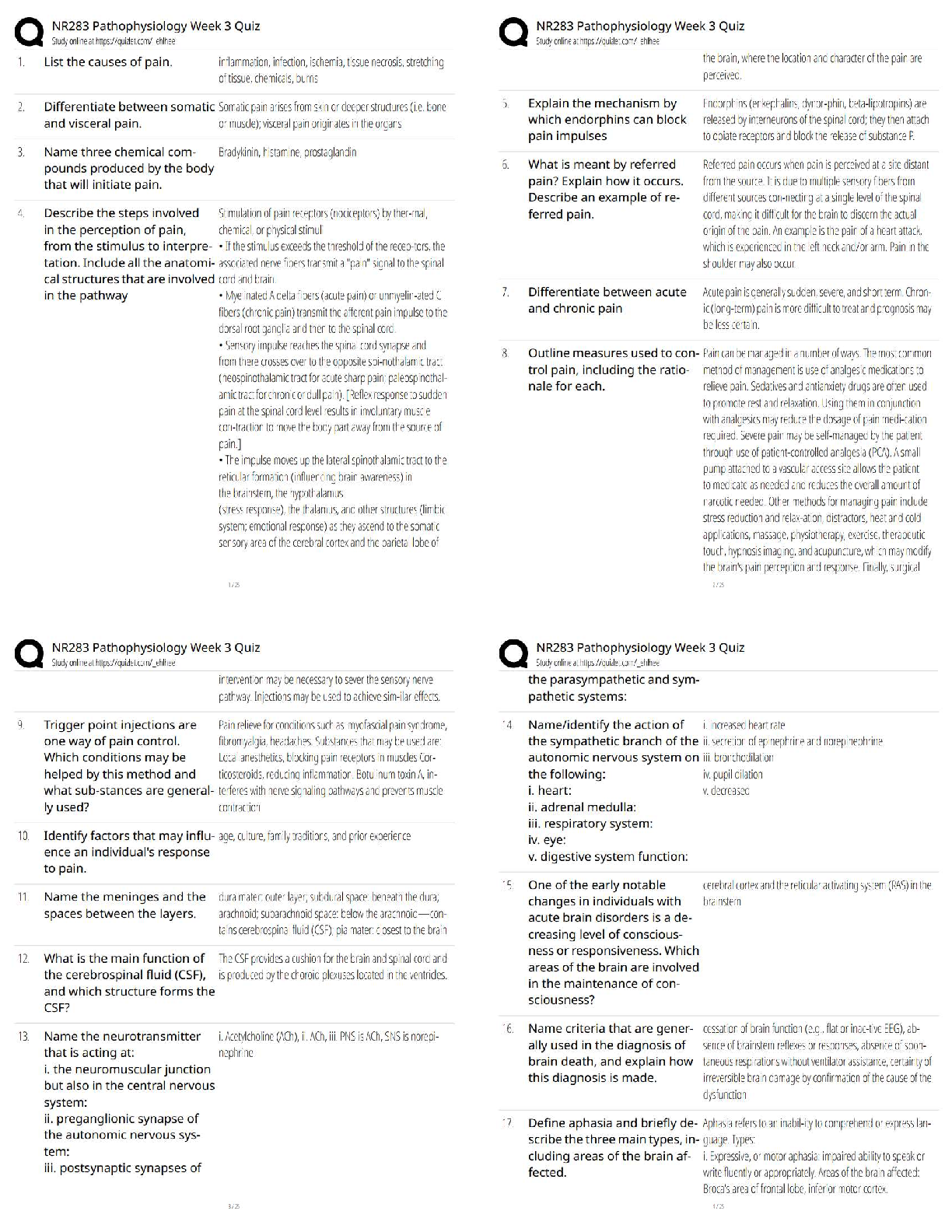


.png)
.png)
.png)